Paper Menu >>
Journal Menu >>
 I. J. Communications, Network and System Sciences, 2008, 2, 105-206 Published Online May 2008 in SciRes (http://www.SRPublishing.org/journal/ijcns/). Copyright © 2008 SciRes. I. J. Communications, Network and System Sciences, 2008, 2, 105-206 Analysis of Lifetime of Large Wireless Sensor Networks Based on Multiple Battery Levels Ruihua ZHANG1, Zhiping JIA1, Dongfeng YUAN2 1 School of Computer Science and Technology, Shandong University, Jinan 250061, P.R.China 2 School of Information Science and Engineering, Shandong University, Jinan 250100, P.R.China E-mail: 1ruihua_zhang@sdu.edu.cn Abstract Due to the limited transmission range, data sensed by each sensor has to be forwarded in a multi-hop fashion before being delivered to the sink. The sensors closer to the sink have to forward comparatively more messages than sensors at the periphery of the network,and will deplete their batteries earlier. Besides the loss of the sensing capabilities of the nodes close to the sink, a more serious consequence of the death of the first tier of sensor nodes is the loss of connectivity between the nodes at the periphery of the network and the sink; it makes the wireless networks expire. To alleviate this undesired effect and maximize the useful lifetime of the network, we investigate the energy consumption of different tiers and the effect of multiple battery levels, and demonstrate an attractively simple scheme to redistribute the total energy budget in multiple battery levels by data traffic load. We show by theoretical analysis, as well as simulation, that this substantially improves the network lifetime. Keywords: Wireless Sensor Networks, Energy Efficient, Network Lifetime, Battery Level 1. Introduction Sensor network applications have recently become of significant interest due to cheap single-chip transceivers and micro-controllers. Because sensor nodes are battery- powered, and their operational lifetime should be maximized, one of the most important design criteria for this type of network is energy efficiency. Confirming the importance of the problem, many aspects of the problem have been extensively studied [1– 4]. Medium access control (MAC) layer techniques [2] [3] aim to conserve battery energy by turning the receiver off whenever it is not needed. It is clear that the energy problem cannot be completely solved at any one single layer [4]. The motivation for our work stems from the observation that in a sensor network, the sensor nodes closer to the sink have to relay more packets than the ones at the periphery of the network. We assume that this increase in workload results in an increase in energy consumption, the nodes close to the sink will die first, leading to a premature loss of connectivity in the sensor network. To alleviate this undesirable effect, we study the energy consumption of different tiers, and demonstrate a scheme to redistribute the total energy budget for the sensor network, the lifetime of the network can be significantly improved over the case where all sensors have a uniform lifetime. The optimal solution is formulated theoretically and validated via simulations. About this problem, in [5–9], non-uniform node deployment is exploited as an alternative manner to get over the effect of non-uniform energy depletion. The basic concept is that different node densities are assigned to different sub-regions trying to balance the communication load of each sub-region. Some works specifically consider the scenario for concentric sub- regions (rings); the node density of a ring is determined based on the number of hops to the sink, which is roughly approximated to be the same for all locations in a ring in [5–7]. In [8], the imbalanced energy utilization of a WSN was analyzed based on the hop counts, and the authors accordingly proposed a non-uniform node distribution depending on the hop-count to improve the long-term connectivity. In [9], the energy-hole problem was discussed in a more general form for a rectangular sensing area with multiple data sinks at different 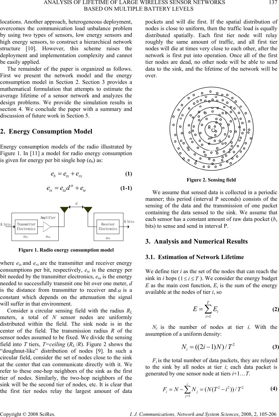 ANALYSIS OF LIFETIME OF LARGE WIRELESS SENSOR NETWORKS 137 BASED ON MULTIPLE BATTERY LEVELS Copyright © 2008 SciRes. I. J. Communications, Network and System Sciences, 2008, 2, 105-206 locations. Another approach, heterogeneous deployment, overcomes the communication load unbalance problem by using two types of sensors, low energy sensors and high energy sensors, to construct a hierarchical network structure [10]. However, this scheme raises the deployment and implementation complexity and cannot be easily applied. The remainder of the paper is organized as follows. First we present the network model and the energy consumption model in Section 2. Section 3 provides a mathematical formulation that attempts to estimate the average lifetime of a sensor network and analyzes the design problems. We provide the simulation results in section 4. We conclude the paper with a summary and discussion of future work in Section 5. 2. Energy Consumption Model Energy consumption models of the radio illustrated by Figure 1. In [11] a model for radio energy consumption is given for energy per bit single hop (eb) as: btxrx eee=+ (1) tx tate eede α =+ (1-1) eta Transmitter Electronics Amplifier eteeta Receiver Electronics K bitsK bits d erx Figure 1. Radio energy consumption model where etx and erx are the transmitter and receiver energy consumptions per bit, respectively, ete is the energy per bit needed by the transmitter electronics, eta is the energy needed to successfully transmit one bit over one meter, d is the distance from transmitter to receiver and α is a constant which depends on the attenuation the signal will suffer in that environment. Consider a circular sensing field with the radius RL meters, a total of N sensor nodes are uniformly distributed within the field. The sink node is in the center of the field. The transmission radius R of the sensor nodes assumed to be fixed. We divide the sensing field into T tiers, T=ceiling (RL /R). Figure 2 shows the “doughnut-like” distribution of nodes [9]. In such a circular field, consider the set of nodes close to the sink at the center that can communicate directly with it. We refer to these one-hop neighbors of the sink as the first tier of nodes. Similarly, the two-hop neighbors of the sink will be the second tier of nodes, etc. It is clear that the first tier nodes relay the largest amount of data pockets and will die first. If the spatial distribution of nodes is close to uniform, then the traffic load is equally distributed spatially. Each first tier node will relay roughly the same amount of traffic, and all first tier nodes will die at times very close to each other, after the network is first put into operation. Once all of the first tier nodes are dead, no other node will be able to send data to the sink, and the lifetime of the network will be over. Figure 2. Sensing field We assume that sensed data is collected in a periodic manner; this period (interval P seconds) consists of the sensing of the data and the transmission of one packet containing the data sensed to the sink. We assume that each sensor has a constant amount of raw data pocket (bs bits) to sense and send in interval P. 3. Analysis and Numerical Results 3.1. Estimation of Network Lifetime We define tier i as the set of the nodes that can reach the sink in i hops (1iT ≤ ≤). We consider the energy budget E as the main cost function, Ei is the sum of the energy available at the nodes of tier i, so 1 T i i EE = = ∑ (2) Ni is the number of nodes at tier i. With the assumption of a uniform density: 2 ((21)) / i NiNT=− (3) Fi is the total number of data packets, they are relayed to the sink by all nodes at tier i; each data packet is generated by one sensor node at tiers i+1…T. 22 2 1 (( ))/ i ij j FNNNT iT = =− =− ∑ (4)  138 R.H. ZHANG ET AL. Copyright © 2008 SciRes. I. J. Communications, Network and System Sciences, 2008, 2, 105-206 In tier i, nodes relay all data pockets generated by nodes at tiers () j ijT<≤ , and nodes at i tier generate and send all data pockets , let Erelay and Egen denote their energy consumed, respectively; es is the energy spent sensing per bit; bs is data pocket size. So we get the relation with energy consumption and time t. irelay gen E EE=+ (5-1) (/ ) relayisb E tpFbe= (5-2) (/ )() g eni sstx E tpNbe e=+ (5-3) Thus 22 2 (()()(21)) sbs tx i tNb eTieei ETp −++− = (5) Li is the lifetime of the nodes at tier i, it can be determined by considering the energy consumption. Using (5), we can get: 2 22 (()(2 1)()) i i sb stx EPT L N bTieie e =−+−+ (6) In accordance with all the above considerations, we define the lifetime of the network as the minimum of the lifetimes of its tiers: 1... min i iT L L = = (7) In this case, each node will start with the same energy, namely E/N; then, the energy at each tier is 2 (2 1) i i NE iE E N T − == (8) Hence, (6) becomes 22 () 21 i s bsstx EP LTi N beNb ee i =−++ − (9) Since the term (T2-i2)/(2i-1) is monotonously decreasing with i for1iT≤≤ , Li the lifetime of tier i is monotonously increasing with i. In other words, the lifetime of the network L is equal to the lifetime of the first tier: 12 (1)() s bsstx EP LL N TbeNbee == −+ + (10) It is obvious that when the lifetime of the first tier has expired, the whole network has expired; the nodes in other tiers have still remaining energy. Using (8) and (9), the residual energy of other tiers Erest: 22 22 ()(21)() [(2 1)] (1) bstx resi bstx Tiei ee E Ei TTeee −+−+ =−− −++ (11) The above equations can also help us determine a reasonable energy allocation for all nodes. One possible criterion is to let the all tiers have the same-targeted lifetime. Thus by balancing energy allocation, by using (2) and (6), we can maximize the network lifetime for a given fixed amount of energy E. 12 T L LL = =⋅⋅⋅= (12) So we get the relation: 22 12 ()(21)() (1) bstx i bstx Tiei ee EE Teee −+−+ =−++ (13) Using (2) and (12), we get the relation: 2 132 2 (( 1)) (43)/ 6() bstx bstx TeeeE ETTTe Tee −++ =−−+ + (14) If we allocate the energies at different tiers according as (13) and (14), we can maximize the network lifetime; all tiers’ energies will be depleted at the same time. 3.2. Design Problems From the above, how to allocate the energies in different tiers is practical importance to the network designers. A reasonable alternative problem specification would provide, instead of the total budget E, the uniform battery level bu for each node. In that case, the lifetime of the network would be independent of the total number of nodes N. The only topology relevant quantity would be the number of tiers T. It will be useful in nodes energy allocation. According to (10), it is obvious that when the lifetime of the first tier and, therefore, the whole network has expired, the nodes in other tiers have still not expended their battery energy. The energy consumption for nodes at different tiers can be easily obtained from a consideration of (10) and (11). The hypothetical lifetime of tier i is Li; but, it is actually expending energy for only the lifetime L of the network. After that, communication stops, and there is no more expenditure of energy. Thus, the ratio of battery energy i e bactually consumed by a node in tier i to the uniform battery level bu that it started with is: i 22 e1 i2 ui () L21 L(1) bstx bstx Ti eee bi CbTeee −++ − === −++ (15) We call the ratios Ci the ideal allocation ratios, because ideally each node would be allocated only the amount of battery it would actually consume during the lifetime. The farther out a node, the lower the fraction Ci of its battery that it has consumed. The unconsumed energy is wastage of the total energy budget. The broad design goal is to redistribute this energy budget non- uniformly so as to increase the lifetime of the whole 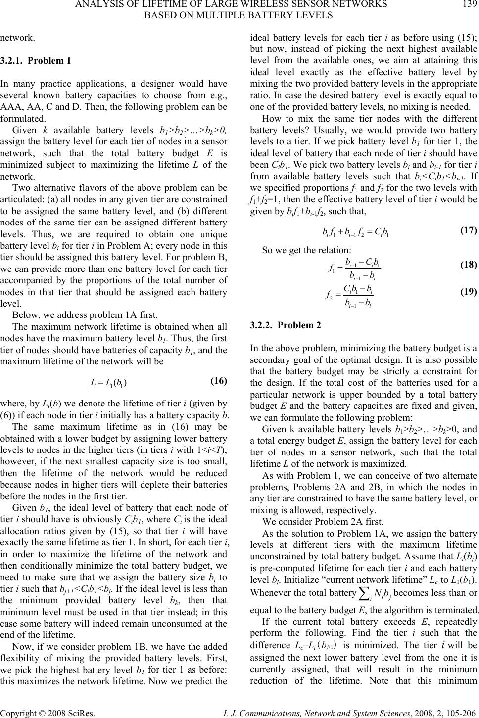 ANALYSIS OF LIFETIME OF LARGE WIRELESS SENSOR NETWORKS 139 BASED ON MULTIPLE BATTERY LEVELS Copyright © 2008 SciRes. I. J. Communications, Network and System Sciences, 2008, 2, 105-206 network. 3.2.1. Problem 1 In many practice applications, a designer would have several known battery capacities to choose from e.g., AAA, AA, C and D. Then, the following problem can be formulated. Given k available battery levels b1>b2>…>bk>0, assign the battery level for each tier of nodes in a sensor network, such that the total battery budget E is minimized subject to maximizing the lifetime L of the network. Two alternative flavors of the above problem can be articulated: (a) all nodes in any given tier are constrained to be assigned the same battery level, and (b) different nodes of the same tier can be assigned different battery levels. Thus, we are required to obtain one unique battery level bi for tier i in Problem A; every node in this tier should be assigned this battery level. For problem B, we can provide more than one battery level for each tier accompanied by the proportions of the total number of nodes in that tier that should be assigned each battery level. Below, we address problem 1A first. The maximum network lifetime is obtained when all nodes have the maximum battery level b1. Thus, the first tier of nodes should have batteries of capacity b1, and the maximum lifetime of the network will be 11 () L Lb= (16) where, by Li(b) we denote the lifetime of tier i (given by (6)) if each node in tier i initially has a battery capacity b. The same maximum lifetime as in (16) may be obtained with a lower budget by assigning lower battery levels to nodes in the higher tiers (in tiers i with 1<i<T); however, if the next smallest capacity size is too small, then the lifetime of the network would be reduced because nodes in higher tiers will deplete their batteries before the nodes in the first tier. Given b1, the ideal level of battery that each node of tier i should have is obviously Cib1, where Ci is the ideal allocation ratios given by (15), so that tier i will have exactly the same lifetime as tier 1. In short, for each tier i, in order to maximize the lifetime of the network and then conditionally minimize the total battery budget, we need to make sure that we assign the battery size bj to tier i such that bj+1<Cib1<bj. If the ideal level is less than the minimum provided battery level bk, then that minimum level must be used in that tier instead; in this case some battery will indeed remain unconsumed at the end of the lifetime. Now, if we consider problem 1B, we have the added flexibility of mixing the provided battery levels. First, we pick the highest battery level b1 for tier 1 as before: this maximizes the network lifetime. Now we predict the ideal battery levels for each tier i as before using (15); but now, instead of picking the next highest available level from the available ones, we aim at attaining this ideal level exactly as the effective battery level by mixing the two provided battery levels in the appropriate ratio. In case the desired battery level is exactly equal to one of the provided battery levels, no mixing is needed. How to mix the same tier nodes with the different battery levels? Usually, we would provide two battery levels to a tier. If we pick battery level b1 for tier 1, the ideal level of battery that each node of tier i should have been Cib1. We pick two battery levels bi and bi-1 for tier i from available battery levels such that b i<Cib1<bi-1. If we specified proportions f1 and f2 for the two levels with f1+f2=1, then the effective battery level of tier i would be given by bif1+bi-1f2, such that, 1121ii i bfbfCb − + = (17) So we get the relation: 11 1 1 ii ii bCb fbb − − − =− (18) 1 2 1 ii ii Cb b fbb − − = − (19) 3.2.2. Problem 2 In the above problem, minimizing the battery budget is a secondary goal of the optimal design. It is also possible that the battery budget may be strictly a constraint for the design. If the total cost of the batteries used for a particular network is upper bounded by a total battery budget E and the battery capacities are fixed and given, we can formulate the following problem: Given k available battery levels b1>b2>…>bk>0, and a total energy budget E, assign the battery level for each tier of nodes in a sensor network, such that the total lifetime L of the network is maximized. As with Problem 1, we can conceive of two alternate problems, Problems 2A and 2B, in which the nodes in any tier are constrained to have the same battery level, or mixing is allowed, respectively. We consider Problem 2A first. As the solution to Problem 1A, we assign the battery levels at different tiers with the maximum lifetime unconstrained by total battery budget. Assume that Li(bj) is pre-computed lifetime for each tier i and each battery level bj. Initialize “current network lifetime” Lc to L1(b1). Whenever the total batteryij iNb ∑ becomes less than or equal to the battery budget E, the algorithm is terminated. If the current total battery exceeds E, repeatedly perform the following. Find the tier i such that the difference Lc–Li( b j +1) is minimized. The tier iwill be assigned the next lower battery level from the one it is currently assigned, that will result in the minimum reduction of the lifetime. Note that this minimum 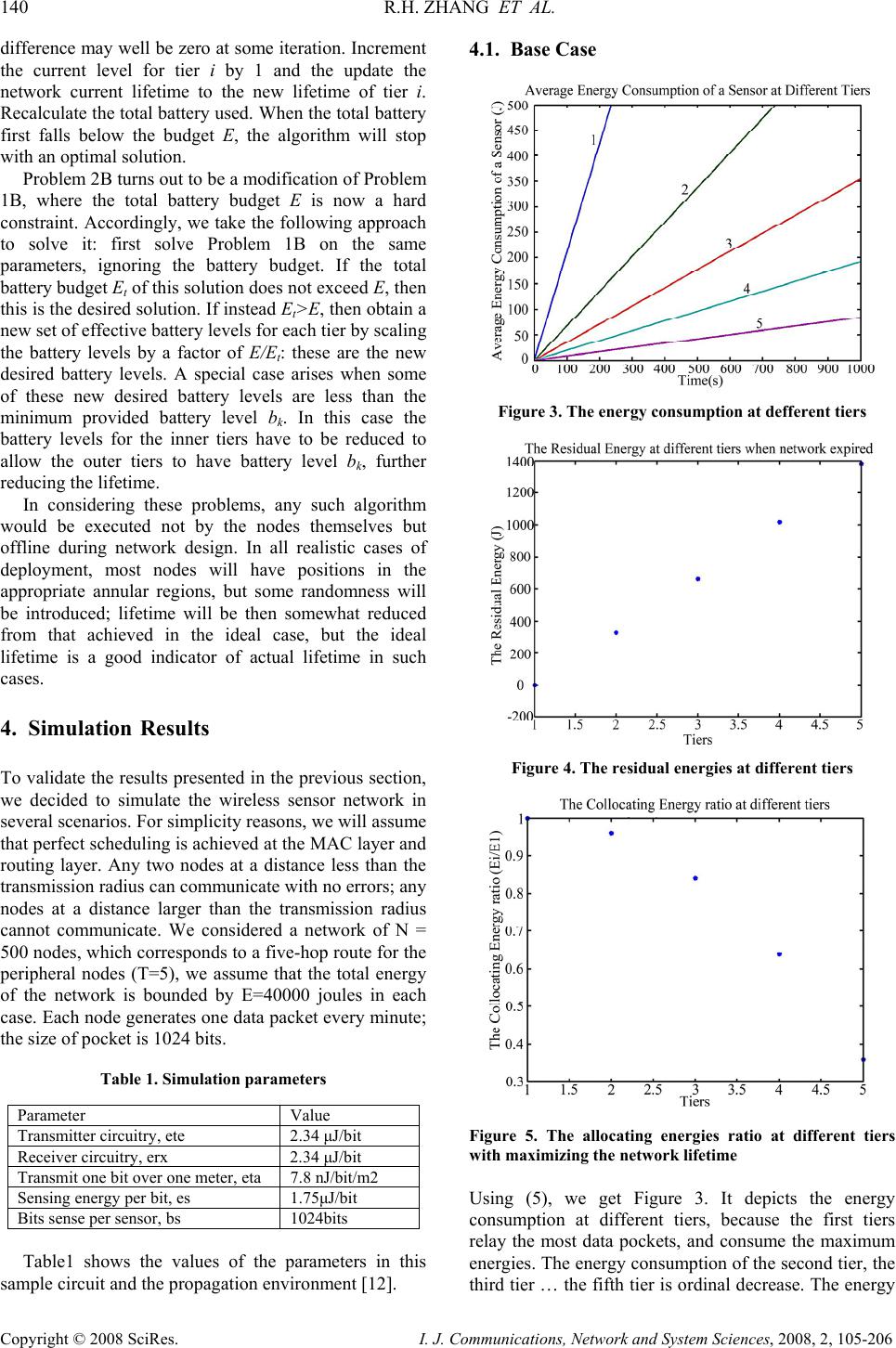 140 R.H. ZHANG ET AL. Copyright © 2008 SciRes. I. J. Communications, Network and System Sciences, 2008, 2, 105-206 difference may well be zero at some iteration. Increment the current level for tier i by 1 and the update the network current lifetime to the new lifetime of tier i. Recalculate the total battery used. When the total battery first falls below the budget E, the algorithm will stop with an optimal solution. Problem 2B turns out to be a modification of Problem 1B, where the total battery budget E is now a hard constraint. Accordingly, we take the following approach to solve it: first solve Problem 1B on the same parameters, ignoring the battery budget. If the total battery budget Et of this solution does not exceed E, then this is the desired solution. If instead Et>E, then obtain a new set of effective battery levels for each tier by scaling the battery levels by a factor of E/Et: these are the new desired battery levels. A special case arises when some of these new desired battery levels are less than the minimum provided battery level bk. In this case the battery levels for the inner tiers have to be reduced to allow the outer tiers to have battery level b k, further reducing the lifetime. In considering these problems, any such algorithm would be executed not by the nodes themselves but offline during network design. In all realistic cases of deployment, most nodes will have positions in the appropriate annular regions, but some randomness will be introduced; lifetime will be then somewhat reduced from that achieved in the ideal case, but the ideal lifetime is a good indicator of actual lifetime in such cases. 4. Simulation Results To validate the results presented in the previous section, we decided to simulate the wireless sensor network in several scenarios. For simplicity reasons, we will assume that perfect scheduling is achieved at the MAC layer and routing layer. Any two nodes at a distance less than the transmission radius can communicate with no errors; any nodes at a distance larger than the transmission radius cannot communicate. We considered a network of N = 500 nodes, which corresponds to a five-hop route for the peripheral nodes (T=5), we assume that the total energy of the network is bounded by E=40000 joules in each case. Each node generates one data packet every minute; the size of pocket is 1024 bits. Table 1. Simulation parameters Parameter Value Transmitter circuitry, ete 2.34 µЈ/bit Receiver circuitry, erx 2.34 µЈ/bit Transmit one bit over one meter, eta 7.8 nЈ/bit/m2 Sensing energy per bit, es 1.75µЈ/bit Bits sense per sensor, bs 1024bits Table1 shows the values of the parameters in this sample circuit and the propagation environment [12]. 4.1. Base Case Figure 3. The energy consumption at defferent tiers Figure 4. The residual energies at different tiers Figure 5. The allocating energies ratio at different tiers with maximizing the network lifetime Using (5), we get Figure 3. It depicts the energy consumption at different tiers, because the first tiers relay the most data pockets, and consume the maximum energies. The energy consumption of the second tier, the third tier … the fifth tier is ordinal decrease. The energy 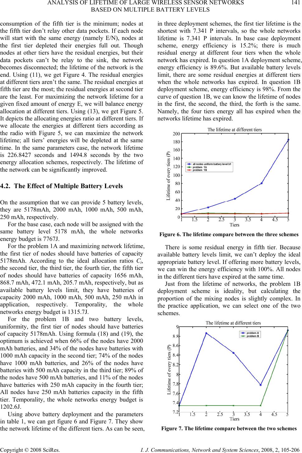 ANALYSIS OF LIFETIME OF LARGE WIRELESS SENSOR NETWORKS 141 BASED ON MULTIPLE BATTERY LEVELS Copyright © 2008 SciRes. I. J. Communications, Network and System Sciences, 2008, 2, 105-206 consumption of the fifth tier is the minimum; nodes at the fifth tier don’t relay other data pockets. If each node will start with the same energy (namely E/N), nodes at the first tier depleted their energies full out. Though nodes at other tiers have the residual energies, but their data pockets can’t be relay to the sink, the network becomes disconnected; the lifetime of the network is the end. Using (11), we get Figure 4. The residual energies at different tiers aren’t the same. The residual energies at fifth tier are the most; the residual energies at second tier are the least. For maximizing the network lifetime for a given fixed amount of energy E, we will balance energy allocation at different tiers. Using (13), we get Figure 5. It depicts the allocating energies ratio at different tiers. If we allocate the energies at different tiers according as the radio with Figure 5, we can maximize the network lifetime; all tiers’ energies will be depleted at the same time. In the same parameters case, the network lifetime is 226.8427 seconds and 1494.8 seconds by the two energy allocation schemes, respectively. The lifetime of the network can be significantly improved. 4.2. The Effect of Multiple Battery Levels On the assumption that we can provide 5 battery levels, they are 5178mAh, 2000 mAh, 1000 mAh, 500 mAh, 250 mAh, respectively. For the base case, each node will be assigned with the same battery level 5178 mAh, the whole networks energy budget is 7767J. For the problem 1A and maximizing network lifetime, the first tier of nodes should have batteries of capacity 5178mAh. According to the ideal allocation ratios Ci, the second tier, the third tier, the fourth tier, the fifth tier of nodes should have batteries of capacity 1656 mAh, 868.7 mAh, 472.1 mAh, 205.7 mAh, respectively, but as available battery levels limit, they have batteries of capacity 2000 mAh, 1000 mAh, 500 mAh, 250 mAh in application, respectively. Temporality, the whole networks energy budget is 1315.7J. For the problem 1B and two battery levels, uniformity, the first tier of nodes should have batteries of capacity 5178mAh. Using formula (18) and (19), the optimum is achieved when 66% of the nodes have 2000 mAh batteries, and 34% of the nodes have batteries with 1000 mAh capacity in the second tier; 74% of the nodes have 1000 mAh batteries, and 26% of the nodes have batteries with 500 mAh capacity in the third tier; 89% of the nodes have 500 mAh batteries, and 11% of the nodes have batteries with 250 mAh capacity in the fourth tier; All nodes have 250 mAh batteries capacity in the fifth tier. Temporality, the whole networks energy budget is 1202.6J. Using above battery deployment and the parameters in table 1, we can get figure 6 and Figure 7. They show the network lifetime of the different tiers. As can be seen, in three deployment schemes, the first tier lifetime is the shortest with 7.341 P intervals, so the whole networks lifetime is 7.341 P intervals. In base case deployment scheme, energy efficiency is 15.2%; there is much residual energy at different four tiers when the whole network has expired. In question 1A deployment scheme, energy efficiency is 89.6%. But available battery levels limit, there are some residual energies at different tiers when the whole networks has expired. In question 1B deployment scheme, energy efficiency is 98%. From the curve of question 1B, we can know the lifetime of nodes in the first, the second, the third, the forth is the same. Namely, the four tiers energy all has expired when the networks lifetime has expired. Figure 6. The lifetime compare between the three schemes There is some residual energy in fifth tier. Because available battery levels limit, we can’t deploy the ideal appropriate battery level. If offering more battery levels, we can win the energy efficiency with 100%. All nodes in the different tiers have expired at the same time. Just from the lifetime of networks, the problem 1B deployment scheme is ideality, but calculating the proportion of the mixing nodes is slightly complex. In the practice application, we can select one of the two schemes. Figure 7. The lifetime compare between the two schemes 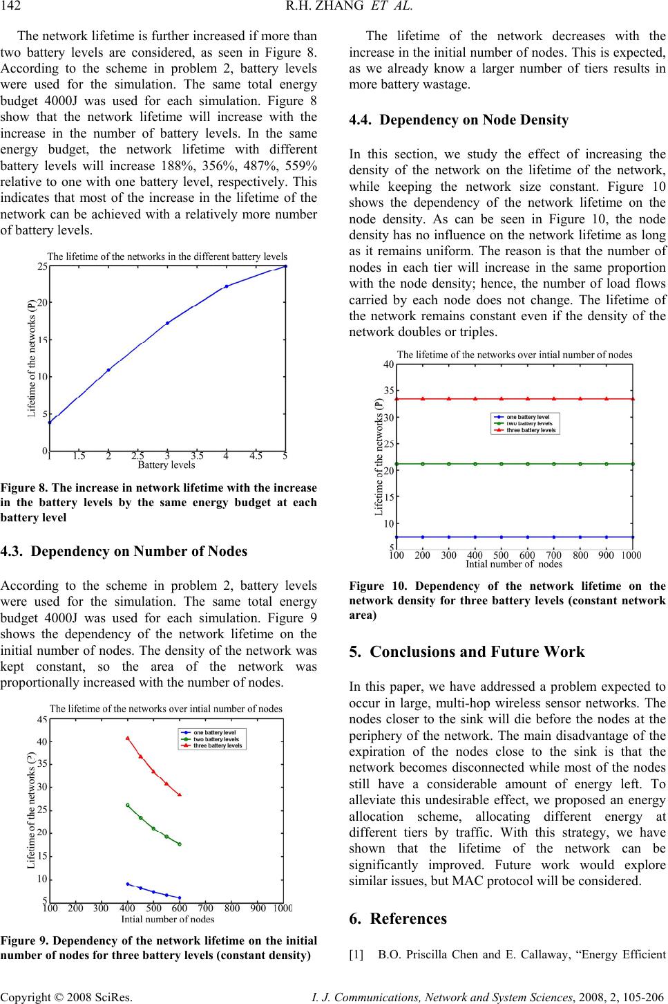 142 R.H. ZHANG ET AL. Copyright © 2008 SciRes. I. J. Communications, Network and System Sciences, 2008, 2, 105-206 The network lifetime is further increased if more than two battery levels are considered, as seen in Figure 8. According to the scheme in problem 2, battery levels were used for the simulation. The same total energy budget 4000J was used for each simulation. Figure 8 show that the network lifetime will increase with the increase in the number of battery levels. In the same energy budget, the network lifetime with different battery levels will increase 188%, 356%, 487%, 559% relative to one with one battery level, respectively. This indicates that most of the increase in the lifetime of the network can be achieved with a relatively more number of battery levels. Figure 8. The increase in network lifetime with the increase in the battery levels by the same energy budget at each battery level 4.3. Dependency on Number of Nodes According to the scheme in problem 2, battery levels were used for the simulation. The same total energy budget 4000J was used for each simulation. Figure 9 shows the dependency of the network lifetime on the initial number of nodes. The density of the network was kept constant, so the area of the network was proportionally increased with the number of nodes. Figure 9. Dependency of the network lifetime on the initial number of nodes for three battery levels (constant density) The lifetime of the network decreases with the increase in the initial number of nodes. This is expected, as we already know a larger number of tiers results in more battery wastage. 4.4. Dependency on Node Density In this section, we study the effect of increasing the density of the network on the lifetime of the network, while keeping the network size constant. Figure 10 shows the dependency of the network lifetime on the node density. As can be seen in Figure 10, the node density has no influence on the network lifetime as long as it remains uniform. The reason is that the number of nodes in each tier will increase in the same proportion with the node density; hence, the number of load flows carried by each node does not change. The lifetime of the network remains constant even if the density of the network doubles or triples. Figure 10. Dependency of the network lifetime on the network density for three battery levels (constant network area) 5. Conclusions and Future Work In this paper, we have addressed a problem expected to occur in large, multi-hop wireless sensor networks. The nodes closer to the sink will die before the nodes at the periphery of the network. The main disadvantage of the expiration of the nodes close to the sink is that the network becomes disconnected while most of the nodes still have a considerable amount of energy left. To alleviate this undesirable effect, we proposed an energy allocation scheme, allocating different energy at different tiers by traffic. With this strategy, we have shown that the lifetime of the network can be significantly improved. Future work would explore similar issues, but MAC protocol will be considered. 6. References [1] B.O. Priscilla Chen and E. Callaway, “Energy Efficient 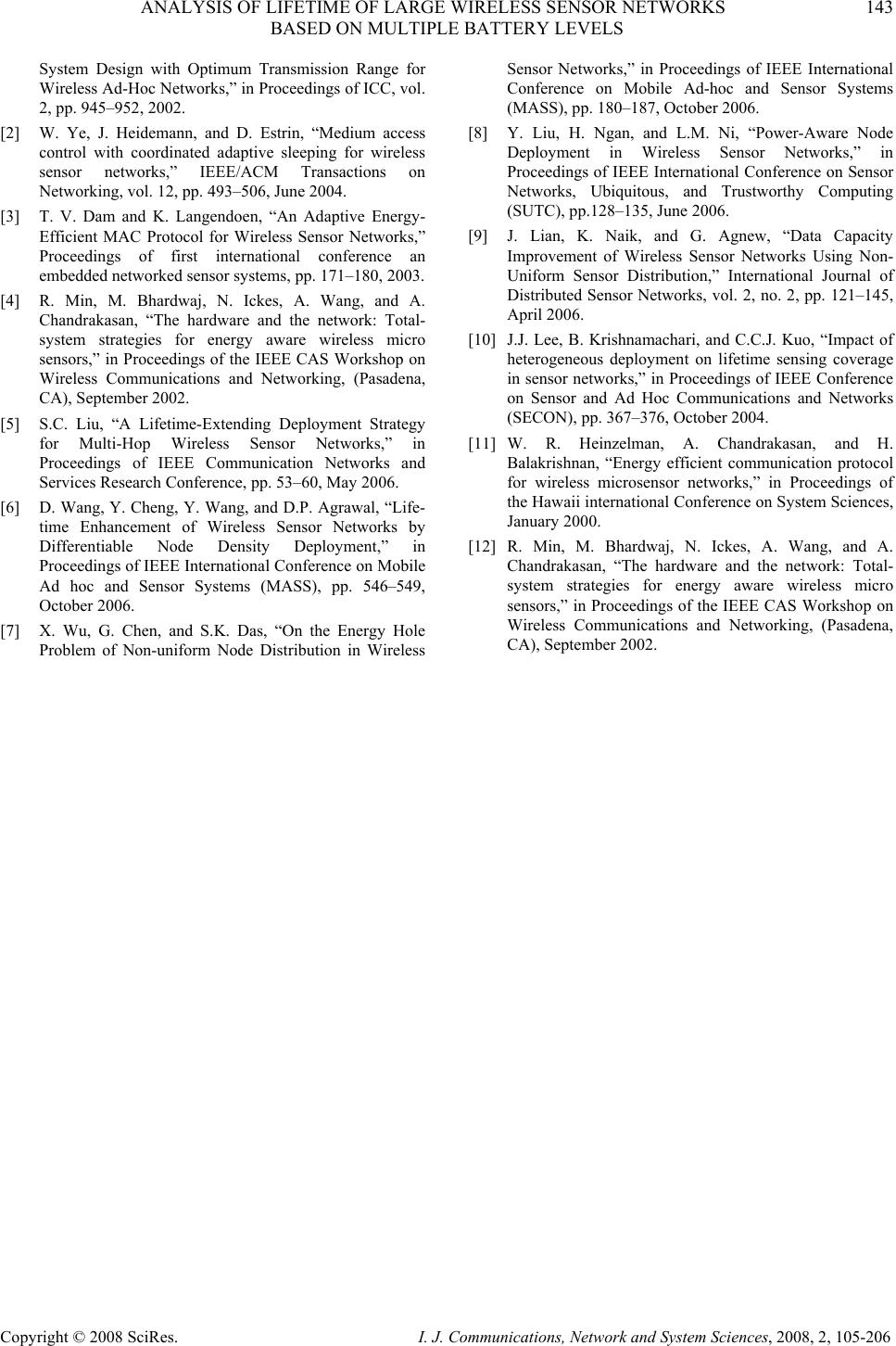 ANALYSIS OF LIFETIME OF LARGE WIRELESS SENSOR NETWORKS 143 BASED ON MULTIPLE BATTERY LEVELS Copyright © 2008 SciRes. I. J. Communications, Network and System Sciences, 2008, 2, 105-206 System Design with Optimum Transmission Range for Wireless Ad-Hoc Networks,” in Proceedings of ICC, vol. 2, pp. 945–952, 2002. [2] W. Ye, J. Heidemann, and D. Estrin, “Medium access control with coordinated adaptive sleeping for wireless sensor networks,” IEEE/ACM Transactions on Networking, vol. 12, pp. 493–506, June 2004. [3] T. V. Dam and K. Langendoen, “An Adaptive Energy- Efficient MAC Protocol for Wireless Sensor Networks,” Proceedings of first international conference an embedded networked sensor systems, pp. 171–180, 2003. [4] R. Min, M. Bhardwaj, N. Ickes, A. Wang, and A. Chandrakasan, “The hardware and the network: Total- system strategies for energy aware wireless micro sensors,” in Proceedings of the IEEE CAS Workshop on Wireless Communications and Networking, (Pasadena, CA), September 2002. [5] S.C. Liu, “A Lifetime-Extending Deployment Strategy for Multi-Hop Wireless Sensor Networks,” in Proceedings of IEEE Communication Networks and Services Research Conference, pp. 53–60, May 2006. [6] D. Wang, Y. Cheng, Y. Wang, and D.P. Agrawal, “Life- time Enhancement of Wireless Sensor Networks by Differentiable Node Density Deployment,” in Proceedings of IEEE International Conference on Mobile Ad hoc and Sensor Systems (MASS), pp. 546–549, October 2006. [7] X. Wu, G. Chen, and S.K. Das, “On the Energy Hole Problem of Non-uniform Node Distribution in Wireless Sensor Networks,” in Proceedings of IEEE International Conference on Mobile Ad-hoc and Sensor Systems (MASS), pp. 180–187, October 2006. [8] Y. Liu, H. Ngan, and L.M. Ni, “Power-Aware Node Deployment in Wireless Sensor Networks,” in Proceedings of IEEE International Conference on Sensor Networks, Ubiquitous, and Trustworthy Computing (SUTC), pp.128–135, June 2006. [9] J. Lian, K. Naik, and G. Agnew, “Data Capacity Improvement of Wireless Sensor Networks Using Non- Uniform Sensor Distribution,” International Journal of Distributed Sensor Networks, vol. 2, no. 2, pp. 121–145, April 2006. [10] J.J. Lee, B. Krishnamachari, and C.C.J. Kuo, “Impact of heterogeneous deployment on lifetime sensing coverage in sensor networks,” in Proceedings of IEEE Conference on Sensor and Ad Hoc Communications and Networks (SECON), pp. 367–376, October 2004. [11] W. R. Heinzelman, A. Chandrakasan, and H. Balakrishnan, “Energy efficient communication protocol for wireless microsensor networks,” in Proceedings of the Hawaii international Conference on System Sciences, January 2000. [12] R. Min, M. Bhardwaj, N. Ickes, A. Wang, and A. Chandrakasan, “The hardware and the network: Total- system strategies for energy aware wireless micro sensors,” in Proceedings of the IEEE CAS Workshop on Wireless Communications and Networking, (Pasadena, CA), September 2002. |