Modern Economy, 2011, 2, 77-83
doi:10.4236/me.2011.22012 Published Online May 2011 (http://www.SciRP.org/journal/me)
Comparativ e Statics of Oligopoly Equilibrium in a Pure
Exchange Economy
Somdeb Lahiri
SPM, PD Petroleum University, Gujarat, India
Received January 25, 2011; revised March 1, 2011; accepted March 29, 2011
Abstract
In this paper we consider an oligopoly an d we are concerned with the effect o f entry in the market of buyers
and/or sellers on the price of the good being sold and the pay-offs/utilities of t he buyers and seller s. The ma-
jor results obtained in this paper are the following: 1) Given the number of buyers both individual as well as
aggregate offers go up as the number of sellers increases. Further, the price of Y decreases, each buyer is
better off and each seller is worse off as the n umber of sellers incr eases. 2) Given the number of sellers, the
price of Y increases, each buy er is worse o ff and each seller is b etter off as th e number of buyers in creases. 3)
As the economy is replicated the equilibrium price decreases. The sequence of equilibrium prices thus ob-
tained converges to the competitive equilibrium price of the original economy. 4) As the economy is repli-
cated the buyers are better off. The sequence of consumption bundles of the buyers converges to the con-
sumption bundle of the buyers at the competitive equilibrium of the original economy. 5) As the economy is
replicated the sellers are worse off. The sequence of consumption bundles of the sellers converges to the
consumption bundle of the sellers at the competitive equilibrium of the original economy.
Keywords: Oligopoly, Pure Exchange, Comparative Statics, Entry-Exit, Replication
1. Introduction
We consider a general equilibrium model with two goods,
i.e. money (X) and an infinitely divisible good (Y),
where buyers are initially endowed only with X and sel-
lers are initially endowed only with Y. Unlike the per-
fectly competitive model we assume that sellers behave
strategically. However where buyers are concerned, they
may or may not behave strategically. If buyers also be-
have strategically then we have a simple version of a
strategic market game due to Shubik [1], Shapley [2] and
Shapley and Shubik [3] that is discussed in Gabszewicz
and Michel [4]. The latter class of models has been stu-
died in [5]. If they act as price-takers then the pure ex-
change economy becomes a version of Counot’s model
of oligopoly. Such models have been discussed in [6].
In this paper we consider an oligopoly and we are
concerned with the effect of entry in the market of buy-
ers and/or sellers on the price of Y and the payoffs/utili-
ties of the buyers and sellers. An increase in the number
of buyers leads to an increase in the availability of X as
also an increase in the demand for Y; an increase in the
number of sellers leads to an increase in the availability
of Y as also an increase in the demand for X. Hence our
paper is concerned with comparative statics in oligopo-
listic markets. Amir and Bloch [7] discuss these issues in
a very general model for bilateral oligopolies. We dis-
cuss similar issues for an oligopoly assuming that buyers
and sellers have Cobb-Douglas utility functions. Hence
whereas our buyers are price takers in the Cournotian
tradition, in the kind of bilateral oligo poly that Amir and
Bloch [7] deal with, buyers behave strategically and
submit bids against the offers that sellers place at the
trading post. Thus the two market structures are entirely
different. Further our use of Cobb-Douglas utility func-
tions allows us to obtain sharper results than what Amir
and Bloch [7] do, albeit in a different market structure.
The analysis in Amir and Bloch [7] “focuses on three
questions: When does an increase in the number of buy-
ers result in an increase in the total bids on the market?
In an increase in the equilibrium price of the private
good? In an increase in the equilibrium utility of the sel-
lers?” We address all the above questions and obtain
definite answers for the same; in addition we show that
entry of new buyers lead to a decline in the utility of ex-
isting buyer. We also obtain definite answers for the ef-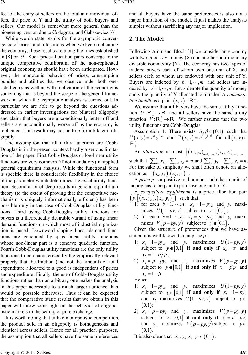

S. LAHIRI
78
fect of the entry of sellers on the total and individual of-
fers, the price of Y and the utility of both buyers and
sellers. Our model is somewhat more general than the
pioneering ve rsi on due t o Codogna to a nd Ga bsz ewi cz [6].
While we do state results for the asymptotic conver-
gence of prices and allocations when we keep replicating
the economy, these results are along the lines established
in [8] or [9]. Such price-allocation pairs converge to the
unique competitive equilibrium of the non-replicated
original economy as should have been anticipated. How-
ever, the monotonic behavior of prices, consumption
bundles and utilities that we observe under both one-
sided entry as well as with replication of the economy is
something that is beyond the scope of the general frame-
work in which the asymptotic analysis is carried out. In
particular we are able to go beyond the questions ad-
dressed in earlier investigations for bilateral oligopoly
and claim that buyers are unconditionally better off and
sellers are unconditionally worse off as the economy is
replicated. This result may not be true for a bilateral oli-
gopoly.
The assumption that all utility functions are Cobb-
Douglas is in the pres ent context hardly a serious limita-
tion of the paper. First Cobb-Douglas or log-linear u tility
functions are very common (if not mandatory) in applied
general equilibrium analysis. While the functional form
is specific there is considerable flexibility in the choice
of the parameter which determines the exact utility fun c-
tion. Second a lot of deep results in general equilibrium
theory (to the extent of proving that the competitive me-
chanism is uniquely informationally efficient) has been
possible only in the case of Cobb-Douglas utility func-
tions. Third using Cobb-Douglas utility functions for
buyers is a theoretically desirable variant of using linear
demand functions on which most of industrial organiza-
tion is based. Downward sloping linear demand func-
tions are generated by quasi-linear utility functions
whose non-linear part is a concave quadratic function.
Fourth Cobb-Douglas utility functions are the only utility
functions to be characterized by the empirically relevant
property that the fraction (and not the amount) of total
expenditure allocated to a good is independent of prices
and expenditure. Finally, the use of Cobb-Douglas utility
functions rather than an arbitrary one makes the analysis
in this paper accessible to a much larger audience than
would be possible otherwise. Thus it can be expected
that the comparative static results that we obtain in this
paper will throw some light on the behavior of oligopo-
listic markets in the setting of pure exchange.
It is worth noting that unlike monopolistic competition,
the product sold in an oligopoly is homogeneous and
identical across sellers. Hence for all practical purposes,
the assumption that all sellers have the same preferences
and all buyers have the same preferences is also not a
major limitation of the model. It just makes the analysis
simpler without sacrif icing any major implication.
2. The Model
Following Amir and Bloch [1] we consider an economy
with two goods i.e. money (X) and another non-monetary
divisible commodity (Y). The economy has two types of
traders: buyers each of whom own one unit of X, and
sellers each of whom are endowed with one unit of Y.
Buyers are indexed by
1, ,bm=
and sellers are in-
dexed by
1, ,sn=
. Let x d enote the quantity of money
and y the quantity of Y allocated to a trader. A consump-
tion bundle is a pair
( )
2
,xy + ∈R.
We assume that all buyers have the same utility func-
tion
2
:U
+
→RR
and all sellers have the same utility
function
2
:V
+
→RR
. We further assume that the two
utility functions are Cobb-Douglas.
Assumption 1: There exists
( )
, 0,1 αβ ∈ such that
( )
1
,U xyxy
αα
−
=
and
( )
1
,V xyxy
ββ −
=
for all
( )
,xy∈
2
+
R
.
An allocation is a list
()( )
1, ,1, ,
, ,,
bb ss
bm sn
xy xy
= =



such that
11 11
and
mn mn
bs bs
bs bs
x xmyyn
= ===
+= +=
∑∑ ∑∑
.
For the sake of simplicity we shall often denote an allo-
cation as
() ()
, ,,
bb ss
xy xy


.
A price p is a positive real number s uch that p units of
money has to be paid to purchase one unit of Y.
A competitive equilibrium is a price allocation pair
() ()
( )
,, ,,
bb ss
p xyxy


such that:
1) for each
1, ,bm=
: 1
bb
x py= − and b y maxi-
mizes
( )
1,Upy y−
subject to
[ ]
0, 1y∈
;
2) for each
1, ,sn=
:
ss
xp py= − and s y maxi-
mizes
( )
,Vppy y− subject to
[ ]
0, 1y∈.
Given the structure of preferences that we have as-
sumed it is well known that at price p:
1) 1
bb
x py= − and b y maximizes
( )
1,Upy y−
subject to
[ ]
0, 1y∈ if and only if
b
x α =
and
1
b
yp α = −
;
2)
ss
xp py= − and s y maxi mi zes
( )
,Vppy y−
subject to
[ ]
0, 1y∈ if and only if s
xp
β = and
1
s
y
β = −.
Hence:
1) 1
bb
x py= − and b y maximizes
( )
1,Upy y−
subject to
[ ]
0, 1y∈ if and only if 1
bb
x py= −
and
b
y
maximizes
( )
1,Upyy−
subject to
y∈
( )
0, 1
;
2)
ss
xp py= − and s y maximizes
( )
,Vppy y−
subject to
[ ]
0, 1y∈ if and only if
ss
xp py
= −
and s
y maximizes
( )
,Vppy y−
subject to
y∈
( )
0, 1
.
It is also clear that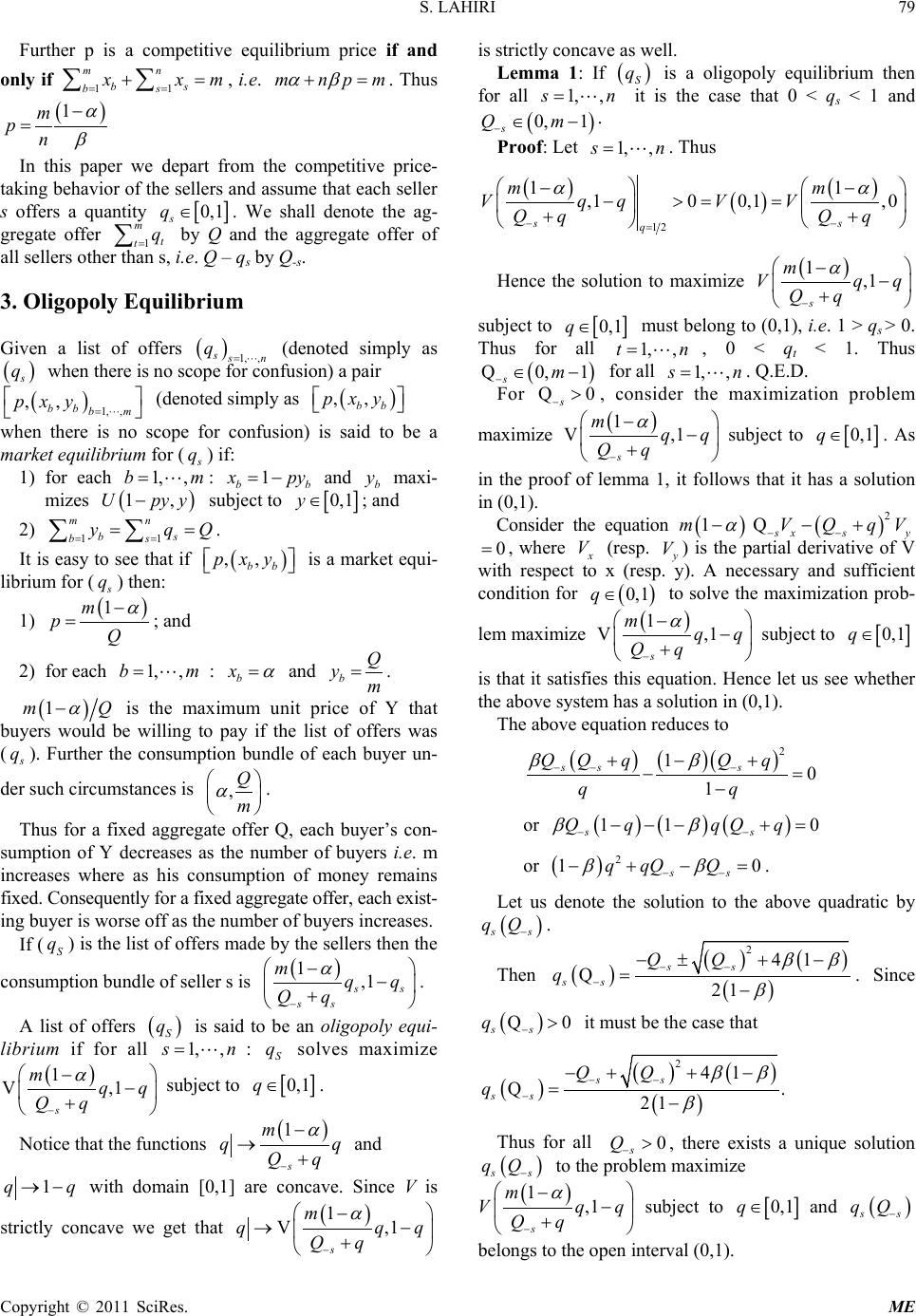
( )
,, ,0,1
bbss
x yxy∈
.

S. LAHIRI
79
Further p is a competitive equilibrium price if and
only if
11
mn
bs
bs
x xm
= =
+=
∑∑
, i.e.
mnpm αβ +=
. Thus
( )
1
m
pn
α
β
−
=
In this paper we depart from the competitive price-
taking behavior of the sellers and assume that each seller
s offers a quantity
[ ]
0, 1
s
q∈
. We shall denote the ag-
gregate offer 1
m
t
tq =
∑ by Q and the aggregate offer of
all sellers other than s, i.e. Q – qs by Q-s.
3. Oligopoly Equilibrium
Given a list of offers
( )
1, ,
s
sn
q= (denoted simply as
( )
s
q
when there is no scope for confusion) a pair
( )
1, ,
,,
bb
bm
pxy =


 (denoted simply as
( )
,,
bb
pxy


when there is no scope for confusion) is said to be a
market equilibrium for (s q) if:
1) for each
1, ,bm=
: 1
bb
x py= − and b y maxi-
mizes
( )
1,Upy y−
subject to
[ ]
0, 1y∈
; and
2)
11
mn
bs
bs
y qQ
= =
= =
∑∑
.
It is easy to see that if
( )
,,
bb
pxy 

is a market equi-
librium for (s q) then:
1)
( )
1m
pQ
α −
=; and
2) for each
1,, bm=
:
b
x α =
and
b
Q
ym =
.
( )
1
mQ
α − is the maximum unit price of Y that
buyers would be willing to pay if the list of offers was
(s
q). Further the consumption bundle of each buyer un-
der such circumstances is ,Q
m
α



.
Thus for a fixed aggregate offer Q, each buyer’s con-
sumption of Y decreases as the number of buyers i.e. m
increases where as his consumption of money remains
fixed. Conse qu e ntly for a fixed aggregate offer, each exist-
ing buyer is worse off as the number of buyers increases.
If (S q) is the list of offers made by the sellers then the
consum ption bundl e of se l ler s is
( )
1,1
ss
ss
mqq
Qq
α
−
− 
−

+

.
A list of offers
( )
S
q is said to be an oligopoly equi-
librium if for all
1,, sn=
: S
q solves maximize
( )
1
V ,1
s
mqq
Qq
α
−
− 
−

+

subject to
[ ]
0, 1q∈.
Notice that the functions
( )
1
s
m
qq
Qq
α
−
−
→+
and
1
qq
→− with domain [0,1] are concave. Since V is
strictly concave we get that
( )
1
V ,1
s
m
q qq
Qq
α
−
−

→−

+

is strictly concave as well.
Lemma 1: If
( )
S
q
is a oligopoly equilibrium then
for all
1,, sn=
it is the case that 0 < qs < 1 and
( )
0, 1
s
Qm
−
∈−
.
Proof: Let
1, ,sn=
. Thus
( )( )( )
12
11
,10 0,1,0
ss
q
mm
VqqV V
Qq Qq
αα
−−
=
−−
 
− >==
 
++
 
Hence the solution to maximize
( )
1,1
s
m
V qq
Qq
α
−
−

−

+

subject to
[ ]
0, 1q∈
must belong to (0,1), i.e. 1 > qs > 0.
Thus for all
1, ,tn=
, 0 < qt < 1. Thus
( )
Q0, 1
sm −
∈−
for all
1, ,sn=
. Q.E.D.
For
Q0
s−>, consider the maximization problem
maximize
( )
1
V ,1
s
mqq
Qq
α
−
− 
−

+

subject to
[ ]
0, 1q∈. As
in the proof of lemma 1, it follows that it has a solution
in (0,1).
Consider the equation
( )
( )
2
1 Q
sx sy
mV QqV α
−−
− −+
0=
, where x V (resp.
y
V
) is the partial derivative of V
with respect to x (resp. y). A necessary and sufficient
condition for
( )
0, 1q∈ to solve the maximization prob-
lem ma xi mi z e
( )
1
V ,1
s
mqq
Qq
α
−
− 
−

+

subject to
[ ]
0, 1q∈
is that it satisfies this equation. Hence let us see whether
the above system has a solution in (0,1).
The above equation reduces to
( ) ( ) ( )
2
10
1
ss s
QQq Qq
qq
ββ
−− −
+− +
−=
−
or
()() ( )
11 0
ss
QqqQ q
ββ
−−
− −−+=
or
( )
2
10
ss
q qQQ
ββ
−−
−+− =
.
Let us denote the solution to the above quadratic by
( )
ss
qQ
−.
Then
( )( )
( )
( )
2
41
Q21
ss
ss
QQ
q
ββ
β
−−
−
−±+ −
=−
. Since
( )
Q0
ss
q
−
>
it must be the case that
( )( )
( )
( )
2
41
Q21
ss
ss
QQ
q
ββ
β
−−
−
−++ −
=−
.
Thus for all
0
s
Q
−
>
, there exists a unique solution
( )
ss
qQ
− to the problem maximize
( )
1,1
s
m
V qq
Qq
α
−
− 
−

+

subject to
[ ]
0, 1q∈ and
( )
ss
qQ
−
belongs to the open interval (0,1).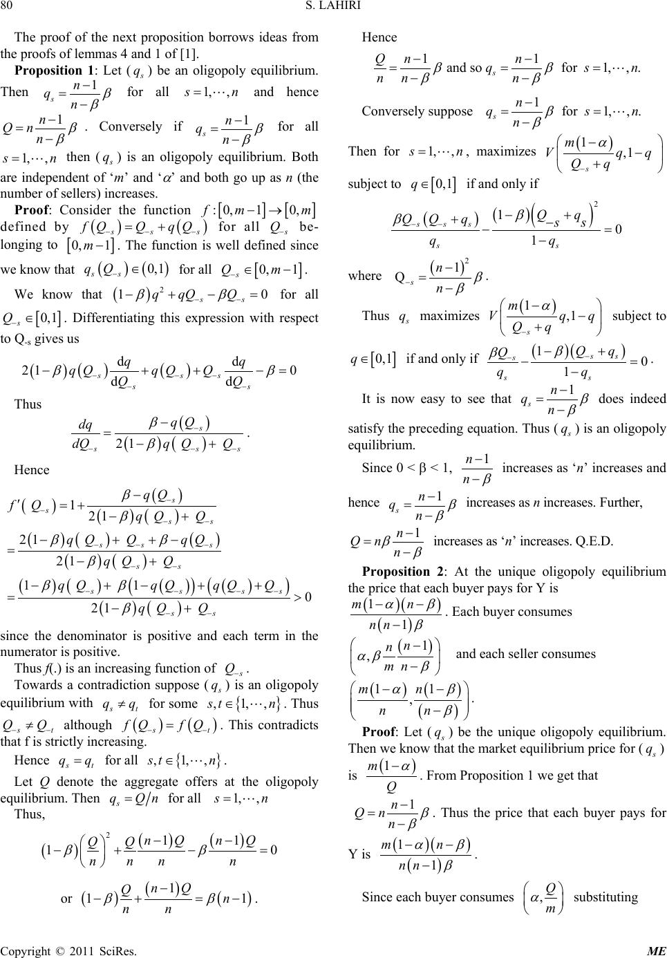

S. LAHIRI
80
The proof of the next proposition borrows ideas from
the proofs of lemmas 4 and 1 of [1].
Proposition 1: Let (s
q
) be an oligopoly equilibrium.
Then
1
s
n
qn β
β
−
=−
for all
1, ,sn=
and hence
1n
Qn
n
β
β
−
=−
. Conversely if
1
s
n
qn β
β
−
=−
for all
1, ,sn=
then (s q) is an oligopoly equilibrium. Both
are independent of ‘m’ and ‘ α ’ and both go up as n (the
number of sellers) increases.
Proof: Consider the function
[] []
: 0,10,fm m−→
defined by
( )( )
ss s
f QQqQ
−− −
= +
for all s
Q
− be-
longing to
[ ]
0, 1m−
. The function is well defined since
we know that
( ) ( )
0, 1
ss
qQ
−
∈
for all
[ ]
0, 1
s
Qm
−
∈−
.
We know that
( )
2
10
ss
q qQQ
ββ
−−
− +−=
for all
[ ]
0, 1
s
Q−∈. Differentiating this expression with respect
to Q-s gives us
( )
( )( )
dd
21 0
dd
s ss
ss
qq
qQqQ Q
QQ
ββ
− −−
−−
−+ +−=
Thus
( )
( ) ( )
21
s
s ss
qQ
dq
dQq QQ
β
β
−
− −−
−
=−+
.
Hence
( )
( )
( )
( )
( )
()( )
( ) ( )
( ) ()( ) ( ) ( ) ( )
( ) ( )
121
21
21
1 10
21
s
sss
ss s
ss
ss ss
ss
qQ
fQ qQ Q
q QQqQ
qQ Q
q QqQqQQ
qQ Q
β
β
ββ
β
ββ
β
−
−
−−
−− −
−−
−− −−
−−
−
′= +−+
−++−
=−+
−+− + +
= >
−+
since the denominator is positive and each term in the
numerator is positive.
Thus f(.) is an increasing function of s
Q−.
Towards a contradiction suppose (s q) is an oligopoly
equilibrium with
st
qq≠
for some
{ }
,1, ,st n∈. Thus
st
QQ
−−
≠ although
()( )
st
fQ fQ
−−
=
. This contradicts
that f is strictly increasing.
Hence
st
qq=
for all
{ }
,1, ,st n∈.
Let Q denote the aggregate offers at the oligopoly
equilibrium. Then s q Qn= for all
1,,sn=
Thus,
( )
( )( )
2
11
10
nQ nQ
QQ
n nnn
ββ
−−

−+− =


or
() ( )( )
1
11
nQ
Qn
nn
ββ
−
−+ =−
.
Hence
11
and so for 1,,.
s
Qn n
q sn
nn n
ββ
ββ
−−
== =
−−

Conversely suppose
1
for 1,,.
s
n
q sn
n
β
β
−
= =
−
Then for
1, ,sn=
, maximizes
( )
1,1
s
m
V qq
Qq
α
−
− 
−

+

subject to
[ ]
0, 1q∈
if and only if
( )
( )
( )
2
10
1
s ss
ss
Qq
QQ qss
qq
β
β
−− −+
+−
−=
−
where
( )
2
1
Q
s
n
n
β
β
−
−
=−
.
Thus s q maximizes
( )
1,1
s
m
V qq
Qq
α
−
−

−

+

subject to
[ ]
0, 1q∈ if and only if
( ) ( )
10
1
ss
s
ss
Qq
Q
qq
β
β
−
−−+
−=
−
.
It is now easy to see that
1
s
n
qn β
β
−
=−
does indeed
satisfy the p receding equation. Thus (s
q) is an oligopoly
equilibrium.
Since 0 < β < 1,
1n
n
β
−
−
increases as ‘n’ increases and
hence
1
s
n
qn β
β
−
=−
i ncreases as n increases. Further,
1n
Qnn ββ
−
=−
i ncreases as ‘n’ increase s. Q.E.D.
Proposition 2: At the unique oligopoly equilibrium
the price that each buyer pa ys for Y is
( )()
( )
1
1
mn
nn
αβ
β
−−
−
. Each buyer consumes
( )
1
,
n
n
mn
αβ β
− 

−

and each seller consumes
() ()
( )
11
,
mn
nn
αβ
β

−−


−

.
Proof: Let (s q) be the unique oligopoly equilibrium.
Then we kn o w that the market equilibrium price for (s
q)
is
( )
1m
Q
α −
. From Proposition 1 we get that
1
n
Qn
n
β
β
−
=− . Thus the price that each buyer pays for
Y is
( )()
( )
1
1
mn
nn
αβ
β
−−
−.
Since each buyer consumes
,Q
m
α



substituting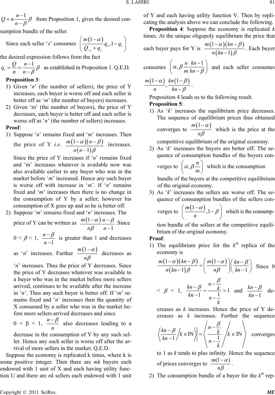

S. LAHIRI
81
1n
Qn
n
β
β
−
=− from Proposition 1, gives the desired con-
sumption bundle of the seller.
Since each seller ‘s’ consumes
( )
1,1
ss
ss
m
qq
Qq
α
−
−

−

+

the desired expression follows from th e f act
1
s
Qn
qnn β
β
−
==− as establi shed in P roposi ti on 1. Q.E.D.
Proposit ion 3:
1) Given ‘n’ (the number of sellers), the price of Y
increases, each buyer is worse off and each seller is
better off as ‘m’ (the number of buy e rs) incr e a se s .
2) Given ‘m’ (the number of buyers), the price of Y
decreases, each buyer is better off and each seller is
worse off as ‘n’ (the number of se l lers) increases.
Proof:
1) Suppose ‘n’ remains fixed and ‘m’ increases. Then
the price of Y i.e.
( )()
( )
1
1
mn
nn
αβ
β
−−
−
increases.
Since the price of Y increases if ‘n’ remains fixed
and ‘m’ increases whatever is available now was
also available earlier to any buyer who was in the
market before ‘m’ increased. Hence any such buyer
is worse off with increase in ‘m’. If ‘n’ remains
fixed and ‘m’ increases then there is no change in
the consumption of Y by a seller; however his
consumption of X goes up and so he is better off.
2) Suppose ‘m’ remains fixed and ‘n’ increases. The
price of Y can be written as
( )
1
1
mn
nn
αβ
β
−−
−
.Since
0 <
β < 1,
1
n
n
β −
−
is greater than 1 and decreases
as ‘n’ increases. Further
( )
1m
n
α
β
−
decreases as
‘n’ increases. Thus the price of Y decreases. Since
the price of Y decreases whatever was available to
a buyer who was in the market before more sellers
arrived, continues to be available after the increase
in ‘n’. Thus any such buyer is better off. If ‘m’ re-
mains fixed and ‘n’ increases then the quantity of
X consumed by a seller who was in the market be-
fore more sellers arrived decreases and since
0 < β < 1,
n
n
β −
also decreases leading to a
decrease in the consumption of Y by any such sel-
ler. Hence any such seller is worse off after the ar-
rival of more sellers in the market. Q.E.D.
Suppose the economy is replicated k times, where k is
some positive integer. Then there are mk buyers each
endowed with 1 unit of X and each having utility func-
tion U and there are nk sellers each endowed with 1 unit
of Y and each having utility function V. Then by repli-
cating the analysis above we can conclude the following.
Proposition 4: Suppose the economy is replicated k
times. At the unique oligopoly equilibrium the price that
each buyer pays for Y is
( )()
( )
1
1
m kn
n kn
αβ
β
−−
−
. Each buyer
consumes
1
,n kn
m kn
αβ β

−

−

and each seller consumes
()()
11
,
m kn
n kn
αβ
β
−−
−.
Proposition 4 leads us to the following result.
Proposit ion 5:
1) As ‘k’ increases the equilibrium price decreases.
The sequence of equilibrium prices thus obtained
converges to
( )
1m
n
α
β
− which is the price at the
competitive equilibrium of the origina l economy.
2) As ‘k’ increases the buyers are better off. The se-
quence of consumption bundles of the buyers con-
verges to ,n
m
αβ



which is the consumption
bundle of the buyers at the competitive equilibrium
of the ori gi na l economy.
3) As ‘k’ increases the sellers are worse off. The se-
quence of consumption bundles of the sellers con-
verges to
( )
1,1 m
n
αβ −

−


which is the consump-
tion bundle of the sellers at the competitive equili-
brium of the original economy.
Proof:
1) The equilibrium price for the kth replica of the
economy is
( )()
( )
( )
11
11
m knmkn
n knnkn
αβα β
ββ
−− − 
−

=

−−

 Since 0
< β < 1,
1
1
1
n
kn k
kn nk
β
β
−
−= >
−−
and
1
kn
kn
β −
− de-
creases as k increases. Hence the price of Y de-
creases as k increases. Further the sequence
IN IN
1
1
n
kn k
kk
kn nk
β
β
−
−∈= ∈
−−
converges
to 1 as k tends to plus infinity. Hence the sequence
of prices converges to
(1 )m
n
α
β
−
.
2) The consumption bundle of a buyer for the kth rep-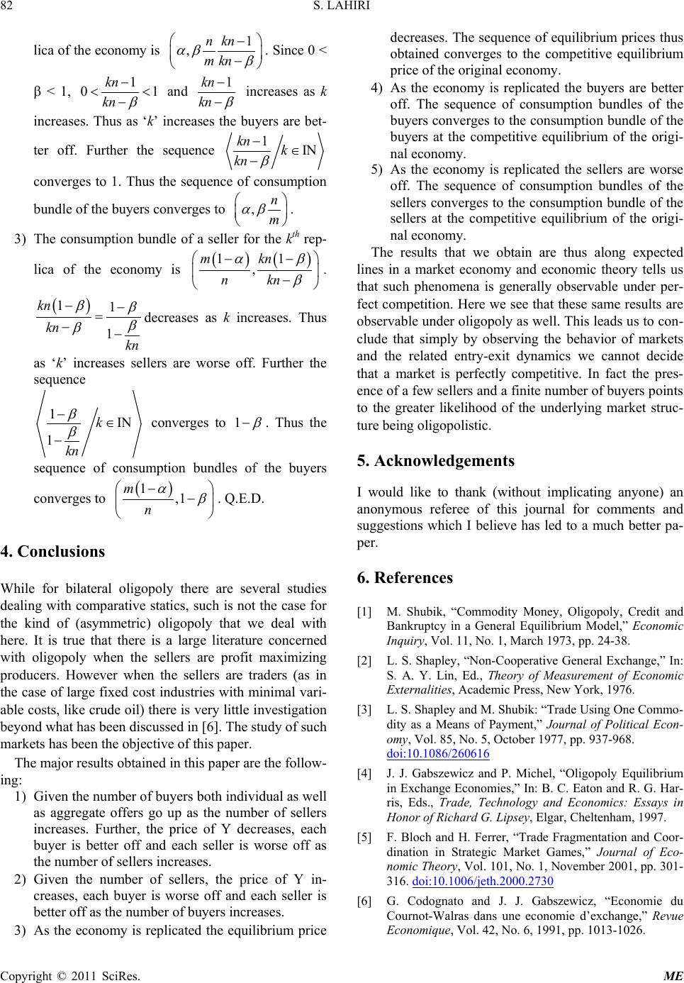

S. LAHIRI
82
lica of the economy is 1 ,n kn
m kn
αβ β

−

−

. Since 0 <
β < 1, 1
01
kn
kn β
−
<<
− and 1
kn
kn β
−
− increases as k
increases. Thus as ‘k’ increases the buyers are bet-
ter off. Further the sequence
1IN kn k
kn
β
−∈
−
converges to 1. Thus the sequence of consumption
bundle of the buyer s converges to
,n
m
αβ



.
3) The consumption bundle of a seller for the kth rep-
lica of the economy is
()()
11
,
m kn
n kn
αβ
β
−− 

−

.
( )
11
1
kn
kn kn
ββ
β
β
−−
=
−−
decreases as k increases. Thus
as ‘k’ increases sellers are worse off. Further the
sequence
1IN
1k
kn
β
β
−∈
−
converges to
1 β −
. Thus the
sequence of consumption bundles of the buyers
converges to
( )
1,1 m
n
αβ − 
−


. Q.E.D.
4. Conclusions
While for bilateral oligopoly there are several studies
dealing with comparative statics, such is not the case for
the kind of (asymmetric) oligopoly that we deal with
here. It is true that there is a large literature concerned
with oligopoly when the sellers are profit maximizing
producers. However when the sellers are traders (as in
the case of large fixed cost industries with minimal vari-
able costs, like crude oil) there is very little i nvestigation
beyond what has been discussed in [6]. The study of such
markets has been the objective of this paper.
The major results obtained in this paper are the follow-
ing:
1) Given the number of buyers both individua l a s w e ll
as aggregate offers go up as the number of sellers
increases. Further, the price of Y decreases, each
buyer is better off and each seller is worse off as
the number of sellers inc reases.
2) Given the number of sellers, the price of Y in-
creases, each buyer is worse off and each seller is
better off as the number of buyers increases.
3) As the economy is replicated the equilibrium price
decreases. The sequence of equilibrium prices thus
obtained converges to the competitive equilibrium
price of the o riginal ec onomy.
4) As the economy is replicated the buyers are better
off. The sequence of consumption bundles of the
buyers converges to the consumption bundle of the
buyers at the competitive equilibrium of the origi-
nal economy.
5) As the economy is replicated the sellers are worse
off. The sequence of consumption bundles of the
sellers converges to the consumption bundle of the
sellers at the competitive equilibrium of the origi-
nal economy.
The results that we obtain are thus along expected
lines in a market economy and economic theory tells us
that such phenomena is generally observable under per-
fect competition. Here we see that these same results are
observable under oligopoly as well. This leads us to con-
clude that simply by observing the behavior of markets
and the related entry-exit dynamics we cannot decide
that a market is perfectly competitive. In fact the pres-
ence of a few sellers and a finite number of buyers points
to the greater likelihood of the underlying market struc-
ture being oligopolistic.
5. Acknowledgements
I would like to thank (without implicating anyone) an
anonymous referee of this journal for comments and
suggestions which I believe has led to a much better pa-
per.
6. References
[1] M. Shubik, “Commodity Money, Oligopoly, Credit and
Bankruptcy in a General Equilibrium Model,” Economic
Inquiry, Vol. 11, No. 1, March 1973, pp. 24-38.
[2] L. S. Shapley, “Non-Cooperative General Exchange,” In:
S. A. Y. Lin, Ed., Theory of Measurement of Economic
Externalities, Academic Press, New York, 1976.
[3] L. S. Shapley and M. Shubik: “Trade Using One Commo-
dity as a Means of Payment,” Journal of Political Econ-
omy, Vol. 85, No. 5, October 1977, pp. 937-968.
doi:10.1086/260616
[4] J. J. Gabszewicz and P. Michel, “Oligopoly Equilibrium
in Exchange Economies,” In: B. C. Eaton and R. G. Har-
ris, Eds., Trade, Technology and Economics: Essays in
Honor of Richard G. Lipsey, Elgar, Cheltenham, 1997.
[5] F. Bloch and H. Ferrer, “Trade Fragmentation and Coor-
dination in Strategic Market Games,” Journal of Eco-
nomic Theory, Vol . 101, No. 1, November 2001, pp. 301-
316. doi:10.1006/jeth.2000.2730
[6] G. Codognato and J. J. Gabszewicz, “Economie du
Cournot-Walras dans une economie d’exchange,” Revue
Economique, Vol. 42, No. 6, 1991, pp. 1013-1026.

S. LAHIRI
83
[7] R. Amir and F. Bloch: “Comparative Statics in a Simple
Class of Strategic Market Games,” Games and Economic
Behavior, Vol. 65, No. 1, 2009, pp. 7-24.
doi:10.1016/j.geb.2007.09.002
[8] S. Lahiri, “Asymptotic Convergence to Competitive
Equilibrium of Oligopoly Equilibria,” 2010.
http://papers.ssrn.com/sol3/papers.cfm?abstract_id=1739
486
[9] R. Lahmandi-Ayed, “Oligopoly Equilibria in Exchange
Economies: A Limit Theorem,” Economic Theory, Vol.
17, No. 3, 2001, pp. 665-674. doi:10.1007/PL00004122