 Journal of Geoscience and Environment Protection, 2014, 2, 15-24 Published Online July 2014 in SciRes. http://www.scirp.org/journal/gep http://dx.doi.org/10.4236/gep.2014.24003 How to cite this paper: Patki, A., Li, X. C., Chen, D., Lou, H., Richmond, P., Damodara, V., Liu, L., Rasel, K., Alphones, A., & Zhou, J. (2014). On Numerical Simulation of Black Carbon (Soot) Emissions from Non-Premixed Flames. Journal of Geo- science and Environment Protection, 2, 15-24. htt p ://dx. doi.org/10. 4236/g ep .2014.24003 On Numerical Simulation of Black Carbon (Soot) Emissions from Non-Premixed Flames Ajit Patki1, Xianchang Li1, Daniel Chen2, Helen Lou2, Peyton Richmond2, Vijaya Dam odara2, Lan Liu2, Kader Rasel2, Arokiaraj Alphones2, Jenny Zhou1 1Department of Mechanical Engineering, Lamar University, Beaumont, TX, USA 2Dan F. Smith Department of Chemical Engineering, Lamar University, Bea umo nt, TX, USA Email: xli2@lamar.edu Received May 2014 Abstract Soot emi ssi ons ( PM 2.5) from land-based sources pose a substantial health risk, and now ar e sub- ject to new an d tougher EPA regulations. Flaring produces significant amo un t of particulate ma tter in the form of soot, alo ng with othe r harmful gas emissions. A few experi ment al studies have pre- viously been done on flames burning in a controlled condition. In these lab-experiments, great ef- fort is needed to collect, sample, and analyz e the soot so that the emiss ion rat e can be calculated. Soot prediction in flares is trick y d ue to variable condit i ons su ch as radiation and surrounding air available for combustion. Work presented in this paper simulates some lab-scale flares in which soot yie ld for methane flame mixture was measured under different conditions. The focus of this paper is on soot modeling with various flair operating conditions. The computati onal fluid dy- namics software ANSYS Fluent 13 is used. Different soot models were explored along with other chemistry mechanisms. The effec t of radiation models, quantity of air supplied, di fferen t fuel mixture and its effect over soot formations were a lso studied. Keywords Numerical Modeling , So ot Em issi on, F lames 1. Introduction Flaring is widely used in many in dustr ies to dispose unwanted combustion gases by burning them. Satellite im- agery analysis suggests more than 139 billion cubic meters of gas were flared worldwide in 2008 [1]. Industrial flares are one of the measure sources of black carbon i.e. soot. Despite the very high amount of gas flared all over the world and the requirement to report associated emissions, an analysis of the very few existing black carbon (PM) emission factors has revealed that current estimation of black carbon production from industrial flares must be interpreted with cautiousness. Soot is considered as a significant health hazard mainly because its small size [2] and it has been linked to serious respiratory, reproductive, and developmental effects in humans [3]. Soot has also been recognized as a significant source of anthropogenic radiative forcin g of the planet’s sur- face [4]-[6]. Measurement of soot emitted by industrial flares with experimental methods is relatively expensive and complex. Johnson et al. [7] in Carleton University, Canada conducted a series of methane mixture flare ex-  A. Patki et al. periments to measure black carbon i.e. soot. These quantitative soot emission measurements were performed on lab-scale flares for a range of burner diameters, exit v elocities and fuel compositions. Computational fluid dynamics (CFD) can be used to predict soot yield from any flare. The key objective of this paper is to simulate a lab-scale flare and analyze the soot data. It is desi red that with a certain soot model the numerical method can reasonably predict the soot yield and eventually help the industrials for flare operation. In this paper, the computational fluid dynamics (CFD) is applied to quantitatively analyze the soot yield f rom non- premixed flames by using basic physics, turbulence and chemist ry models and reliable soot model. The commer- cial software package, ANSYS Fluent 13.0, is used for this purpose. The ef fect of radiatio n models and quantity of air supplied was studied. Soot yield from flame under variable conditions is examined. 2. Governing Equations and S oot Modelin g 2.1. Conser vation Equations The 3D time-averaged steady-state Navi e r-Stokes equations as well as the equations for mass con servation and energy transports need to be solved. In addition, the species transport and chemical reactions need to be cons i- der ed too . Because the time-averaged Nav i er-Stokes equations cannot take the turbulen ce fluctu ation directly, a turbulent model is needed. For industrial application, the k- ε model is one of popular turbulence models. The k- ε model consists of two transport equations , wh ic h need to be solved to compute the Reynold s stresses given by 2 3 j i i jijt ji u u uu kxx ρρδ µ ∂ ∂ ′′=++ ∂∂ (1) where µt is the eddy kinematic viscosity, δij is the Kronecker delta and k is the kinetic energy of turbulence. The and repr esent the fluc tuating ve locity in different directions. The two transport equations of this model can be given as. () () t ik ii ki kk uk G tx xx µ ρρ µρε σ ∂∂ ∂∂ += ++− ∂∂ ∂∂ (2 ) 2 12 () () t ik ii i u CGC txxx kk ε µ ρεε εε ρε µρ σ ∂∂ ∂∂ += +++ ∂∂ ∂∂ (3) where C1, C2, σk and σ ε are empirical constants. Gk is the generation term for turbulence. The turbulent viscosity can be calculated by. (4 ) where the constant Cµ = 0.09. The species equ ation is a statement of conservation of a single species. The c ons ervatio n equation f or the mass fraction ( ) of species is given by '', '' () () ii iiiii ii mumJR S tx x ρρ ′ ∂∂∂ +=− ++ ∂∂ ∂ ( 5) where is the ith component of the diffusion flux of species in the mixture, Ri' is th e net rate of produc- tion of species i' by chemical reaction and Si' is the source term from the dispersed phase or any user defined source. 2.2. Soot Models The Mo s s-Brookes model solves transport equations for normalized radical nuclei concentration and soot mass fraction Ysoot: () () soott soot i soot ii sooti YY dM uY txxx dt ρµ ρσ ∂∂ ∂∂ += + ∂∂∂∂ (6)  A. Patki et al. ** * () 1 () nuct nuc i nuc ii nucinorm bb dN ub txxxN dt ρµ ρσ ∂∂ ∂∂ += + ∂∂∂∂ (7) where Ysoot is soot mass fraction, M is soot mass concentration (kg/m3), is the normalized radical nuclei concentration, and N is soot particle number density (particles/m3). Nnorm = 1015 particles. In the one-step (Khan and Greeves) model, ANSYS Fluent solves a single transport equation for the soot mass fraction: () () soott soot i sootsoot ii sooti YY uY R txxx ρµ ρσ ∂∂ ∂∂ += + ∂∂∂∂ (8) where Ysoot is soot mass fraction, σsoot is turbule nt Prandtl number for soot transport, and Rsoot is net rate of soot generation. The default constants for the one-step model are valid for a wide ran ge of hydrocarbon fuels. The two-step (Tesner) model predicts the generation of radical nuclei and then computes the formation of soot on these nuclei. ANSYS FLUENT therefore solves transport equations for two scalar quantities: the soot mass fraction and the normalized radical nuclei concentration. ** ** () () nuct nuc i nucnuc ii nuci bb ub R txx x ρµ ρσ ∂∂ ∂∂ += + ∂∂∂∂ (9) where is normalized radical nuclei concentration (particles × 10−15/kg), σnuc is the turbulent Prandtl number for nuclei transport, and is the normalized net rate of nuclei generation (particles × 10−15/m3s). In these transport equations, the rates of n uclei and soot generation are the net rates, involving a balance between formation and combustion. More details of the se models as well as the default coefficients can be found in [8]. 2.3. Chemical Mechanisms Numerical simulation of combustion requires a comprehensive reaction kinetics mechanism, which takes care of all the reaction pathways and the species that are produced during and at the end of combustion. CHEMKIN, a reaction engi neeri n g software package, was used to develop the reaction mechanism. The 50-species combustion mechanism termed LU 1.0 was reduced from the combined GRI and USC mechanisms. The combined GRI- USC thermo mechanism consists of 93 species, and has to be further reduced to 50 species to satisfy the maxi- mum species limit set by Fluent. The reduction mechanism was validated by sensitivity and the rate of reaction. The detailed mechanism had 93 species and 600 reactions which were reduced in a step wise manner to 50 spe- cies and 337 reactions. 3. Numerical Modeling 3.1. Comput ational Domain and Mesh In this s tudy, ANS YS Wor kbe nch is u s ed to create the 3D geometry. The concept of flame is sh own in Figu re 1. Air is supplied from the bottom part of cylinder and the fuel inlet is given from stack. The geometry consists of two axially concentric cylinders. One is for main domain and another is for stack inlet. The diameter and height of large cylinder are 0.7 and 2.2 m, respectively, where the diameters and height of stack inlet is 25 mm and 0.2 m, respectively. The outlet is placed at top of the computational domain. The mesh is shown in Figure 2. Circular edges of cylinder are divided into 60 equal parts. Whereas the height above stack is divided into 100 parts with bias factor of 12. Therefore, mesh is denser near stack and less dense away from stack. Side edges near stack are also divided into 26 parts with bias factor of 16. Mesh is denser at center and less dense away from the center. Once the mesh is build, it is checked for mesh orthogonal quality. Orthogonal quality near to unity is considered as good quality. Therefore mesh orthogonal quality of current geometry is monitored and kept above 0.8. The mesh used for simulation consists of 0.22 million cells. The si- mulation was performed on a system with Intel Quad core i5 processors, CPU at 3.2 GHZ and RAM of 8 GB. 3.2. Boundary Conditions and Numerical Procedures The commercial software ANSYS Fluent 13.0 is used for simulation. Gravity is applied in negative Y-axis as 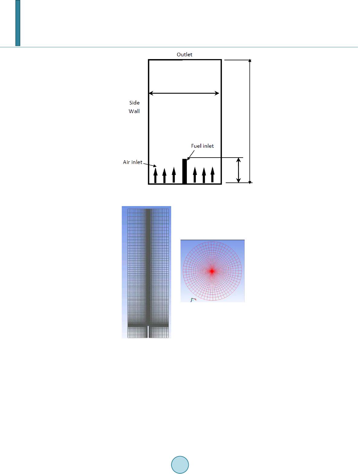 A. Patki et al. Figure 1. Concept of flame and computational domain. Figure 2. Mesh in different views. −9.81 m/s². The standard k-ε model with standard wall functions is used as viscous model. SIMPLE algorithm is enabled for pressure-velocity coupling. The non-premixed combustion species model (PDF model) is used to simulate the combustion process. The CHEMKIN kinetic reaction mechanism file and 93 thermo file are im- ported to the fluent by using CHEMKIN Import. Two types of fuel are considered and the fuel composition is given in Table 1. Mixture 1 is used for most of the cases while Mixture 2 is used to study the effect of fuel composition on soot generation. Once fuel is specified, flamelets are generated until either the maximum number of flamelets is reached or the flamelets are extinguished. Extinguished flamelets are not included in library. In ANSYS Fluent, the flamelets can be either generated by the users or imported from other packages. The parameters used for flamelet genera- tion are listed in Table 2. These parameters are limited by computer memory and a fatal error may occur if the parameters are increased beyond a certain level.  A. Patki et al. Table 1. Fuel composition. Fuel Mixture 1 Mixture 2 CH4 73.00% 91.00% C2H6 12.00% 4.11% C3H8 9.57% 3.00% CO2 3.28% 1.14% N2 2.15% 0.75% Table 2. Flamelet generation parameters. Number of grid points in flamelet 100 Maximum number of flamelets 30 Initial scalar dissipation (1/s) 0.01 Scalar dissipation step (1/s) 5 The grid refinement was used while generating the flamelets. ANSYS Fluent has the option for automated grid refinement of steady flamelets. An adaptive algorithm inserts grid points so that the change of values as well as the change of slopes between successive grid points is less than user specified tolerances. During auto- mated grid refinement, a steady solution is calculated on a coarse grid with a user specified initial number of grid points in flamelets. When it reaches to the convergence, a new grid point is inserted between a point i and its neighbor (i + 1) if it satisfies a certain condition. The parameters for automated grid refinement are listed in Table 3. After the flamelets are generated, the flamelet profiles are convoluted with the assumed-shape PDFs and then tabulated for look-up in ANSYS Fluent. The parameters used to generate the PDF table are listed in Table 4. In addition to those settings described above, the operating pressure, temperature and gravity need to be ap- plied. Before starting each case, the solution was initialized from the co-flow inlet. An iso-surface (Z = 0) paral- lel to X-Y plane was created at the center of domain. The maximum temperature at Z = 0 plane was monitored during iteration. Once the temperature was stabilized and the solution was converged the results were saved for further analysis. The emission is measured at the top surface (outlet) of the domain. 4. Results and Discussion 4.1. Baseline Case By applying the settings explained in above section, the baseline case with 0.5 m/s jet velocity (fuel inlet veloc- ity) is studied first. Air is supplied from the air inlet at 0.25 m/s. After some preliminary studies, the Moss- Brooke soot model is chosen. The radiation effect is not ignored for the baseline case. Figure 3 shows the tem- perature contours along different cross section. It can be said that the highest temperature of the flame is around 1720 K. The height of the flame is approximately 1.1 m. Figure 4 shows the velocity vector and soot fraction contour. Soot is produced approximately 0.5 m above the stack. Its peak is located almost the same as the maximum temperature. To compare the soot formation for dif- ferent cases, flow rate of soot is calculated at the outlet and the flow rate of fuel is calculated at inlet. Soot yield (kg/kg) is calculated by using following formula. flowrateof soot at outlet(kgs) Soot Yieldflow rateoffuelatinlet(kgs) = (10 ) The soot yield as well as other parameters is given in Table 5. 4.2. Effect of Soot Models It is not easy to model the soot generation accurately. Fluent gives three soot models: One-step soot model, two-step soot model, and Moss-Brooks soot model. To explore the difference among these models, all parame- 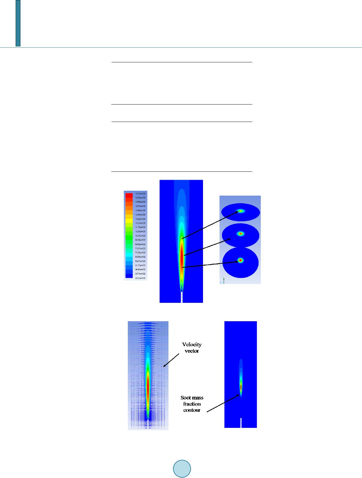 A. Patki et al. Table 3. Grid refinement parameters for flamelet. Initial number of grid points in flamelet 8 Maximum number of grid points in flamelet 64 Maximum change in value ratio 0.5 Maximum change in slope ratio 0.5 Table 4. Parameters used to generate the PDF table. Number of mean mixture fraction points 80 Number of mixture fraction variance points 40 Maximum number of species 19 Number of mean enthalpy points 41 Minimum temperature (k) 298 Figure 3. Temperature contour of the baseline case. Figure 4. Velocity vectors and soot contours of the baseline.  A. Patki et al. ters of the baseline case are kept the same but soot model. Different soot models are applied and soot yield re- sults are presented in Table 6. From results of the flow rate of soot at outlet, it can be said that One-step and two-step soot models give very low values for soot yield. However, the Moss-Brooks model gives a r easonable soot yield, i.e. closer to the experimental results in [7]. 4.3. Effect of Air Velocities It is known that air supply affects the combustion process and thu s the soo t generation. To und erstand h ow im- portant the air supplied is, the baseline case is tried with different air velocities. The temperatu re and soot results are presented in Table 7. From these results, it can be inferred that soot yield also increases as air supplied in- creases. Also there is a slight rise in flame temperature with higher air velocity. 4.4. Effect of Chemical Mechanisms For the chemical reactions, Fluent has an equilibrium option with which no mechanism is needed. In such case, Fluent non-premixed model (i.e. PDF model) uses its own mechanism which contains 20 species. There is no need to use flamelet model if this equilibrium option is taken. To examine the impact of chemical mechanism, the baseline case is repeated with the equilibrium option where the flamelet is not generated. Its results are compared to those with flamelets. As listed in Table 8, the model without mechanism and flamelet gives very low soot yield at outlet. Also the maximum temperature attained by flame is relatively lower than that with flamelet. 4.5. Soot Yield with Different Fuel Mixture To further understand the behavior of soot models in Fluent, the second type of fuel is studied. The details of fuel composition are given earlier in Table 1. The results are compared to the baseline case. As seen in Table 9, soot yield results are significantly lower for Mixture 2, which is because Mixture 2 has more methane (91%) than Mixture 1 (73%). T here is more carbon in Mixture 1 and more carbon means higher potential for soot yield. Also the maximum flame te mperatur e attaine d by Mixture 2 flame is slig h tly lower than that with Mixture 1. 4.6. Effect of Radiation on Soot Yield In all the cases so far, the effect of radiation is neglected. In this section, radiation is considered to examine how it is important to soot yield. As an initial attempt, P-1 radiation model is enabled. The P-1 radiation model is the simplest case of the more general P-N model, which is based on the expansion of the radiation intensity into an orthogonal series of spherical harmonics. The results are presented in Table 10. From Table 10, it is seen that soot yield at the outlet for both cases is almost same. Also, the maximum flame temperature differs only slightly. Therefore, it can be concluded that radiation does not make any big difference in soot yield or the maximum temperature attained by the flame. Table 6. Soot yield results for three different soot models. Soot model Flow rate of soot at outlet (kg/s) Soot yield (kg/kg) One step 1.41 × 10⁻¹² 7.42 × 10⁻⁹ Two step 1.72 × 10⁻¹⁹ 9.05 × 10⁻¹⁶ Moss-Brooke 1.40 × 10⁻⁶ 0.0073 Table 7. Soot yield results for different air velocities. Air velocity (m/s) Soot at outlet (kg/s) Soot yield (kg/kg) Max temp (K) 0.25 1.40 × 10⁻⁶ 0.0073 1720.5 0.5 1.77 × 10⁻⁶ 0.0092 1736.1 0.75 2.20 × 10⁻⁶ 0.0115 1750.8 1 2.83 × 10⁻⁶ 0.0148 1765.1  A. Patki et al. 4.7. Effect of Fuel Jet Velocity To examine the soot formation with different jet velocity or fuel flow rate, five more jet velocities are consi- dered. All the other parameters are kept the same. These jet velocities are 0.1, 0.25, 0.9, 1.5, and 2.2 m/s. Figure 6 shows the temperature contours through the centerline in the vertical direction for all the cases with different jet velocities, and Table 11 gives details of soot yield and flame temperatures. It is observed that height of the flame increased as jet velocity increases due to the big momentum with high velocity. When the velocity is high, the computational domain can be too short to complete all the chemical reactions. In addition, it is observed that the flame temperature increases slightly with increase in jet velocity. However, the rate of soot emission increases significantly when the velocity increases, which is actually against the study by McEwen and Johnson [7]. In their experiments, McEwen and Johnson [7] found that the soot yield reaches a maximum and then drops when the jet velocity further increases. More studies are needed to explore the difference. The contours of soot mass fraction are given in Figure 7, which shows the peak region moves up with increase in jet velocity. 5. Conclusion Based on the numerical results in this study, it can be concluded that, among three different soot models, the Moss-Brooke model provides more reasonable results for methane mixture flame. The study also indicates that when more air is supplied, the soot yield is higher. As expected, results with different fuel mixture advocate that Table 8. Soot yield with different chemical mechanisms. Models Soot flow rate (kg/s) Soot yield (kg/kg) Max temp (K ) Without Flamelet 2.18 × 10⁻⁹ 0.000015 1677.1 With Flamelet 1.40 × 10⁻⁶ 0.007361 1720.5 Table 9. Soot yield for two different fuel mixtures. Fuel Mixture Soot at exit (kg/s) Soot yield (kg/kg) Max temp (K) Mixture 1 (73% CH4) 1.401 × 10⁻⁶ 0.00736 1720.5 Mixture 2 (91% CH4) 1.479 × 10⁻⁷ 0.00074 1697.6 Table 10. Comparison of cases with and without radiation. Model Soot at exit (kg/s) Soot yield (kg/kg) Max temp (K) Without radiation 1.401 × 10⁻⁶ 0.0073 1720.5 With radiation 1.374 × 10⁻⁶ 0.0072 1717.6 Table 11. Soot yield and maximum temperature for different jet velocities. Jet velocity (m/s) Soot yield (kg/kg) Max temperature (K) 0.1 0.0006 1590 0.25 0.0022 1670 0.5 0.0073 1720 0.9 0.0160 1749 1.5 0.0273 1768 2.2 0.0377 1778 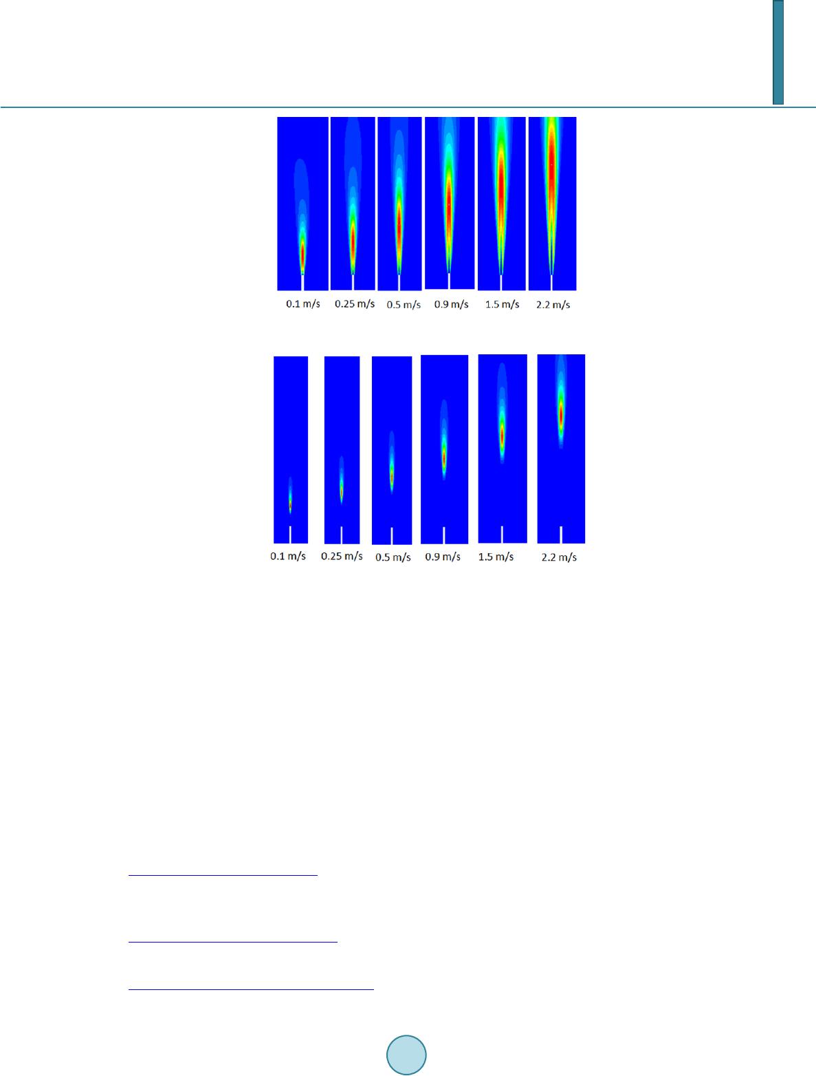 A. Patki et al. Figure 6. Flame temperature with different jet velocities. Figure 7. Soot formation with different jet velocities. soot yield increases as carbon percentage in fuel increases. Furthermore, it can be inferred that, the equilibrium model provided in Fluent produces significantly lower soot yield than LU 1.0 mechanism steady flamelet model. By using P-1 radiation model it is seen that the radiation effect is negligible on methane mixture soot yield and flame temperature. Finally, soot yield results with different jet velocities propose that soot yield increases as jet velocity increases. In the meantime the flame maximum temperature also increases slightly when the jet velocity becomes higher. Acknowledgements This work is partially su pp orted by the Texas Commissio n of Environmental Qu ality and the Texas A ir Re- search Center. References (2010). US EPA Integrated Science Assessment for Particulate Matter EPA/600/R-08/139F. Washington DC. Elvidge, C. D., Ziskin, D., Baugh, K. E., Tuttle, B. T., Ghosh, T., Pack, D. W., Erwin, E. H., & Zhizhin, M. (2009). A Fif- teen Year Record of Global Natural Gas Flaring Derived from Satellite Data. Energies, 2, 595-622. http://dx.doi.org/10.3390/en20300595 Fluent Manual (2006). Version 6.2.36. Fluent, Inc. Hansen, J., Sato, M., Ruedy, R., Lacis, A., & Oinas, V. (2000). Global Warming in the Twenty-First Century: An Alternative Scenario. Proceedings of the National Academy of Sciences of the United States of America, 97, 9875-9880. http://dx.doi.org/10.1073/pnas.170278997 McEwen, J. D. N., & Johnson, M.R. (2012). Black Carbon Particulate Matter Emission Factors for Buoyancy Driven Asso- ciated Gas Flares. Journal of the Air & Waste Management Association, 62, 307-321. http://dx.doi.org/10.1080/10473289.2011.650040  A. Patki et al. Pope III, C. A., Burnett, R. T., Thun, M. J., Eugenia, E. C., Krewski, D., Ito, K., & Thruston, G. D. (2002). Lung Cancer, Cardiopulmonary Mortality, and Long-Term Exposure to Fine Particulate Air Pollution. JAMA: The Journal of the Amer- ican Medical Association, 287, 1132-1141. http://dx.doi.org/10.1001/jama.287.9.1132 Ramanathan, V., & Carmichael, G. (2008). Global and Regional Climate Changes Due to Black Carbon. Nature Geoscience, 1, 221-227. http://dx.doi.org/10.1038/ngeo156 Solomon, S., Qin, D., Manning, M., Chen, Z., Marquis, M., Averyt, K. B., Tignor, M., & Miller, H. L. (2007). Contribution of Working Group I to the Fourth Assessment Report of the Intergovernmental Panel on Climate Change (p. 996). Ca m- bridge: Cambridge University Press.
|