Journal of Modern Physics, 2011, 2, 236-247
doi:10.4236/jmp.2011.24033 Published Online April 2011 (http://www.SciRP.org/journal/jmp)
Analytic algorithms for Some Models of Nonlinear
Age–Structured Population Dynamics and Epidemiology
Vipul K. Baranwal, Ram K. Pandey, Manoj P. Tripathi, Om. P. Singh
Department of Ap pl i e d M athematics, Institute of Technology, Banaras Hindu University,
Varanasi, India
Received January 4, 2011; revised February 7, 2011; accepted February 9, 2011
Abstract
Three analytic algorithms based on Adomian decomposition, homotopy perturbation and homotopy analysis
methods are proposed to solve some models of nonlinear age-structured population dynamics and epidemi-
ology. Truncating the resulting convergent infinite series, we obtain numerical solutions of high accuracy for
these models. Three numerical examples are given to illustrate the simplicity and accuracy of the methods.
Keywords: Age-Structured Population Models, Population Dynamics, SIS Epidemic Models, Adomian
Decomposition Method, Homotopy Perturbation and Homotopy Analysis Methods.
1. Introduction
Individuals in a structured population are distinguished
by age, size, maturity and some other individual physical
characteristics. The basic assumption when modelling
the evaluation of such a population is that the structure of
the population with respect to these individual physical
characteristics at a given time, and possibly some envi-
ronmental inputs as time evolves, completely determines
the dynamical behaviours of the population. Mathemati-
cal models describing this evolution have attracted a
considerable amount of interest among scientists as a
tool for modelling the interaction of different population
communities in such diverse fields as demography, epi-
demiology, ecology, cell kinetics, tumer growth etc.
For a long time, there has been an interest in model-
ling population dynamics. The first discrete population
model appears in Liber Abaci by Leonardo Pisano in
1228 [1], which gives rise to the celebrated Fibonacci
sequences. The simplest continuous model is due to
Malthus in 1798 [2]. His model is an unstructured one
and it leads to an exponential growth of the population
which is usually invalid for large time. Forty years later,
in 1838, Verhulst proposed a logistic model which im-
pose a maximum size for the population by considering
the effects of crowding and the limitation of resources.
In order to build adequate models for population dy-
namics, some detail concerning individual behaviour and
its effects on vital rates of growth, production, and death
must be included. Perhaps the most natural way to con-
sider such effects is to in troduce the age variable in to the
model describing the population dynamics.
Among the first continuous population models incor-
porating age effects were those of Sharpe and Lotka [3]
and McKendrick [4]. Basically, the Sharpe-Lotka-
McKendrick models assume that birth and mortality
processes are linear functions of population density. In
1974, Gurtin and MacCamy [5] proposed a nonlinear age
structured model. The allowed the mortality rate and the
fertility rate to be affected by the total population, which
is true for the most real cases. Their model generalizes
Verhulst’s, and under reasonable assumptions on the
vital rates of the population, results in a logistic model
with bound ed growth.
We consider the following nonlinear age–structured
population model [5] and name it as model (A):
 
,0,0,
uu xPt uxAt
tx

 0,


  (1.1)




0
,0, 0,uxu xxA

 (1.2)
   
0
0,,,d ,0,
A
ut xPtuxtxt 


 (1.3)
 
0
,d, 0,
A
Ptuxtx t


 (1.4)
and some related epidemic models introduced latter,
where


,uxtis the population density (or age-density)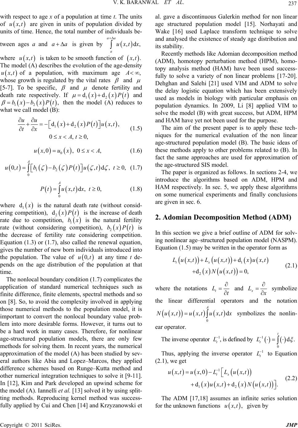

V. K. BARANWAL ET AL.
237
aa
with respect to age x of a population at time t. The units
of are given in units of population divided by
units of time. Hence, the total number of individuals be-

,uxt

ux
tween ages a and is given by

,d,
aa
a
uxt x


where is taken to be smooth function of

,t


,.
x
t
,A
The model (A) describes the evolution of the age-density
of a population, with maximum age

,uxt


whose growth is regulated by the vital rates

and

[5-7]. To be specific,

and

denote fertility and
death rate respectively. If
 


12
dd
x
xPt   and
then the model (A) reduces to
what we call model (B):

bx
 
xPt
12
b, 
 
12
dd ,
0,0,
uu ,
x
xPtuxt
tx xAt

  


 
(1.5)
 
0
,0, 0,uxu xxA


(1.6)
 
12
0
0,,d ,0,
A
utbbPtu tt   


 (1.7)
 
0
,d, 0,
A
Ptuxtx t
 (1.8)
where 1

d
x
is the natural death rate (without consid-
ering competition), 2
 
d
x
Pt is the increase of death
rate due to competition,


bx
1 is the natural fertility
rate (without considering competition),



bxPt
2 is
the decrease of fertility rate considering competition.
Equation (1.3) or (1.7), also called the renewal equation,
gives the number of new born individuals introduced into
the population. The value of at any time t de-
pends on the age distribution of the population at that
time.

0,t

u
The nonlocal boundar y cond ition (1.7) complicates the
application of standard numerical techniques such as
finite difference, finite elements, spectral methods and so
on [8]. So, to avoid the complexity involved in applying
those numerical methods to the population model, it is
important to convert the nonlocal boundary value prob-
lem into more desirable forms. However, it turns out to
be a hard work in many cases. Therefore, for nonlinear
age-structured population models, there are only few
methods for solving them. In recent years, the numerical
approximation of the model (A) has been studied by sev-
eral authors like Abia and Lopez–Marcos, they applied
difference schemes based on Runge–Kutta method and
other numerical integration techniques to solve it [9-11].
In [12], Kim and Park developed an upwind scheme for
the model (A). Iannelli et al. [13] solved it by using sp lit-
ting methods. Reproducing kernel method was success-
fully applied by Cui and Chen [14] and Krzyzanowski et
al. gave a discontinuous Galerkin method for non linear
age structured population model [15]. Norhayati and
Wake [16] used Laplace transform technique to solve
and analysed the existence of steady age distribution and
its stability.
Recently methods like Ado mian decomposition method
(ADM), homotopy perturbation method (HPM), homo-
topy analysis method (HAM) have been used success-
fully to solve a variety of non linear problems [17-20].
Dehghan and Salehi [21] used VIM and ADM to solve
the delay logistic equation which has been extensively
used as models in biology with particular emphasis on
population dynamics. In 2009, Li [8] applied VIM to
solve the model (B) with great success, but ADM, HPM
and HAM have yet not been used for the pur pose.
The aim of the present paper is to apply these tech-
niques for the numerical evaluation of the non linear
age-structured population model (B). The basic ideas of
these methods apply to other problems related to (B). In
fact the same approaches are used for approximation of
the age-structured SIS model.
The paper is organized as follows. In sections 2-4, we
introduce the algorithms based on ADM, HPM and
HAM respectively. In sec. 5, we apply these algorithms
on some numerical experiments and finally conclusions
are given in sec. 6.
2. Adomian Decomposition Method (ADM)
In this section we give a brief outline of ADM for solv-
ing nonlinear age–structured population model (NASPM).
Equation (1.5) may be written in the operator form as







  
 

1
2
,,d
d,0,
tx
Lu xtLu xtxu xt
xNuxt


,
(2.1)
where the notations t
Lt



and x L
x

 symbolize
the linear differential operators and the notation
symbolizes the nonlin-
ear operator.
  
0
,,,
A
Nuxtuxtuxt xd
The i nvers e op erat or 1
t
L

, is de fined by
 
1
0
d
t
t
L



.
Thus, applying the inverse operator to Equation
(2.1), we get
1
t
L



 
  
1
12
,,0,
d,d ,
tx
uxtuxLL uxt
xuxt xNuxt




 .
(2.2)
The ADM [17,18] assumes an infinite series solution
for the unknown functions given by

,,uxt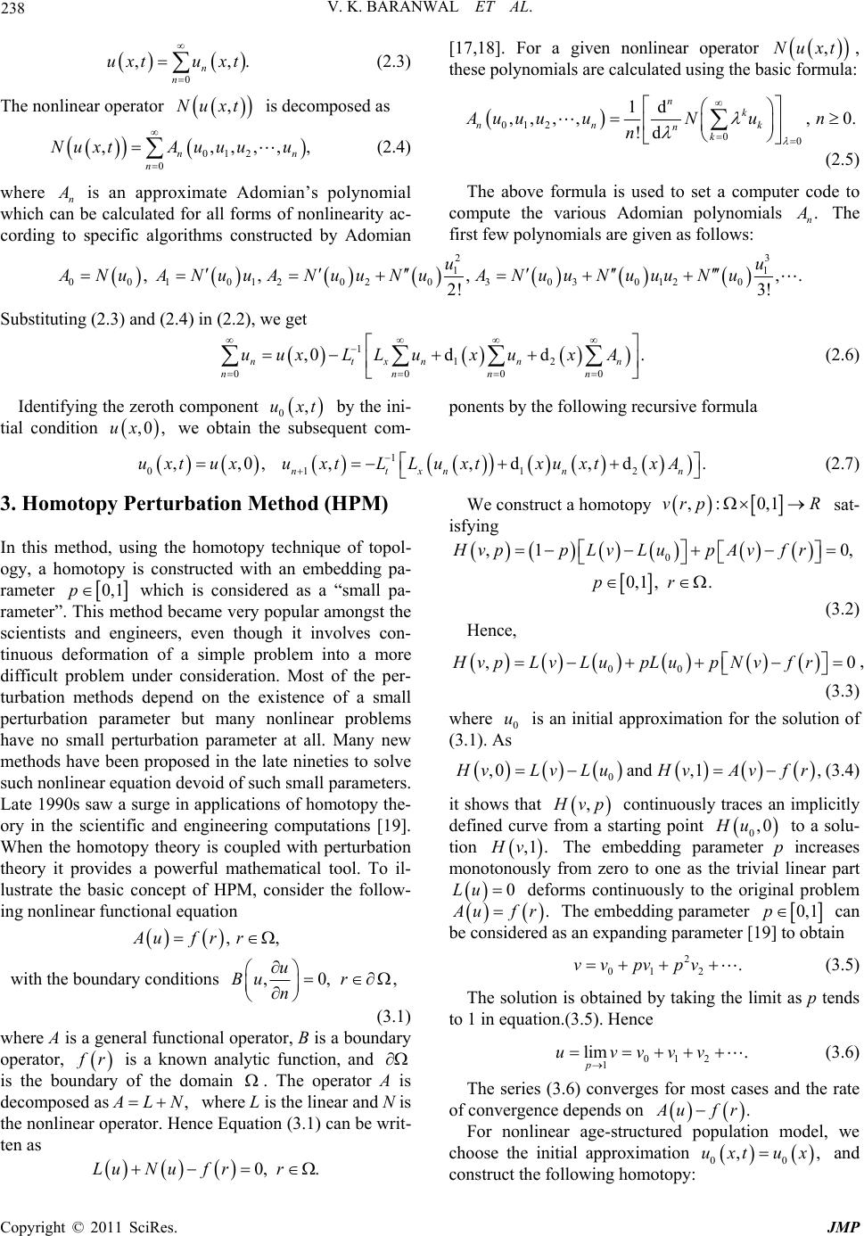

V. K. BARANWAL ET AL.
238
,[17,18]. For a given nonlinear operator




,Nuxt,
these polynomials are calculated using the ba sic formula:
 
0
,
n
n
uxtu xt


. (2.3)
The nonlinear ope rato r



,Nuxt


,,
n
is decomposed as

012 00
1d
,,,,, 0.
!d
nk
nn k
nk
Auuu uNun
n















(2.5)
  
012
0
,,,,
n
n
NuxtAu uuu


 (2.4)
The above formula is used to set a computer code to
compute the various Adomian polynomials .
n
A
The
first few polynomials are given as follows:
where n
A
is an approximate Adomian’s polynomial
which can be calculated for all forms of nonlinearity ac-
cording to specific algorithms constructed by Adomian
 
23
11
00101202 03 03 0120
,, ,
2! 3!
uu
A NuANuuA Nuu NuA NuuNuuu Nu
 
 ,.
0
n
n


Substituting (2.3) and (2.4) in (2.2), we get
  
112
000
,0d d.
ntxnn
nnn
uuxLLux uxA





 





(2.6)
Identifying the zeroth component by the ini-
tial condition we obtain the subsequent com-ponents by the following recursive formula

0,uxt

,0 ,ux












 
1
01 12
,,0,,,d ,d
ntxn n
uxtuxuxtL LuxtxuxtxA

.
n




 (2.7)
We construct a homotopy
 

,: 0,1vrp R sat-
isfying
3. Homotopy Perturbation Method (HPM)





  



0
,1
0,1 ,.
HvppLvLupAvfr
pr

In this method, using the homotopy technique of topol-
ogy, a homotopy is constructed with an embedding pa-
rameter


0,1p which is considered as a “small pa-
rameter”. This method became very popular amongst the
scientists and engineers, even though it involves con-
tinuous deformation of a simple problem into a more
difficult problem under consideration. Most of the per-
turbation methods depend on the existence of a small
perturbation parameter but many nonlinear problems
have no small perturbation parameter at all. Many new
methods have been proposed in the late nineties to solve
such nonlinear equation devoid of such small parameters.
Late 1990s saw a surge in applications of homotopy the-
ory in the scientific and engineering computations [19].
When the homotopy theory is coupled with perturbation
theory it provides a powerful mathematical tool. To il-
lustrate the basic concept of HPM, consider the follow-
ing nonlinear functional eq uation
0,

 
 


(3.2)
Hence,





 


00
,0HvpLvLupLupNvfr

 

,
(3.3)
where 0 is an initial approximation for the solution of
(3.1). As
u





  


0
,0and ,1,
H
vLvLu HvAvfr(3.4)
it shows that


,
H
vp continuously traces an implicitly
defined curve from a starting point to a solu-
tion

0,0Hu



,1Hv . The embedding parameter p increases
monotonously from zero to one as the trivial linear part


0Lu

deforms continuously to the original problem




.
A
ufr The embedding parameter


0, 1p can
be considered as an expanding parameter [19] to obtain
 
,,Auf rr
2
01 2.vvpvpv  (3.5)
with the boundary conditions ,0,
u
Bu r
n





 ,
The solution is obtained by taking the limit as p tends
to 1 in equation.(3.5). Hence
(3.1)
where A is a general functional operator, B is a boundary
operator,

f
r is a known analytic function, and


is the boundary of the domain . The operator A is
decomposed as ,
A
LN where L is the linear and N is
the nonlinear operator. Hence Equation (3.1) can be writ-
ten as
012
1
lim .
p
uvvvv


 (3.6)
The series (3.6) converges for most cases and the rate
of convergence depends on




.
A
ufr
For nonlinear age-structured population model, we
choose the initial approximation



00
,,uxt ux and
construct the following homotopy:
 


0, .LuNuf rr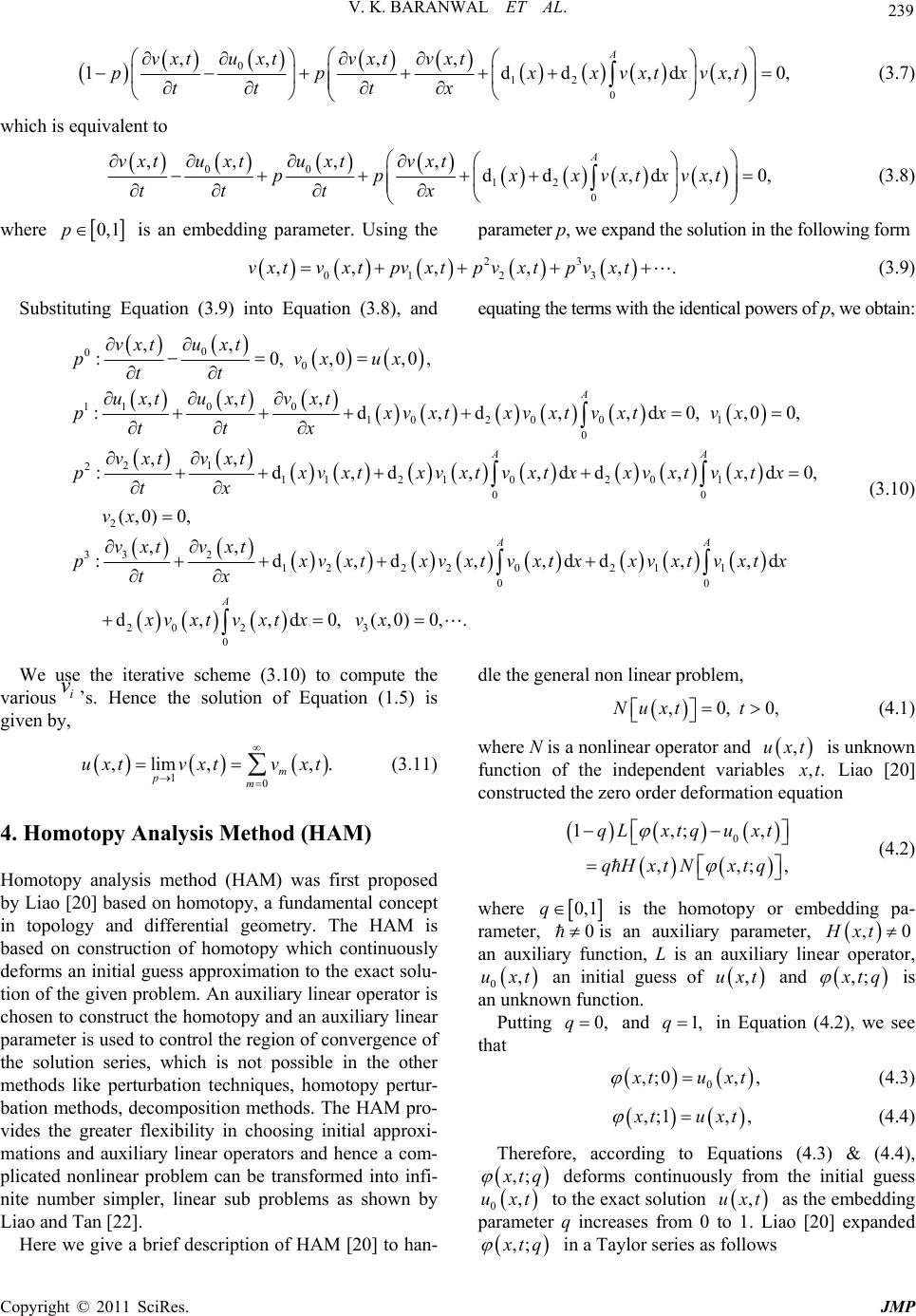

V. K. BARANWAL ET AL.
239

     
012
0
,, ,,
1dd
A
vxtu xtvxtvxt
pp xxvxtx
tt tx

   


 

 
 

,d,0,vxt
(3.7)
which is equivalent to
    
00 12
0
,, , ,
dd ,d,
A
vxtuxtu xtvxt
pp xxvxtxvxt
tt tx

 
  



 


0
,
(3.8)
where


0,1p is an embedding parameter. Using the parameter p, we expand the solution in the following form
 






23
01 2 3
,, ,,,vxt vxt pvxt pvxt pvxt . (3.9)
Substituting Equation (3.9) into Equation (3.8), and eq u a ti ng t h e t er ms w i th th e id e n t i ca l p o w e r s o f p, we obtain:
  
   
  
 
0 00
100 11020 01
0
21 2112102 01
00
2
32 3
,,
:0,,0,0,
,,,
:d,d,,d0,
,,
:d,d,,dd,
(,0)0,
,,
:
A
AA
vxtu xt
pvxux
tt
uxt uxt vxt
pxvxtxvxtvxtx vx
ttx
vxt vxt
pxvxtxvxtvxtxxvxtvxt x
tx
vx
vxt vxt
pt

 





 







,00,
,d0,
 
 
1222021 1
00
20 23
0
d,d,,d d,,d
d,,d0,(,0)0,.
AA
A
xvxtxvxtvxtxxvxtv xtx
x
xvxtvxtxv x
 



(3.10)
We use the iterative scheme (3.10) to compute the
various ’s. Hence the solution of Equation (1.5) is
given by,
i
v
 
10
,lim, ,
m
pm
uxtvxtv xt



. (3.11)
4. Homotopy Analysis Me t h o d (HAM)
Homotopy analysis method (HAM) was first proposed
by Liao [20] based on homotopy, a fundamental concept
in topology and differential geometry. The HAM is
based on construction of homotopy which continuously
deforms an initial guess approximation to the exact solu-
tion of the given problem. An auxiliary linear operator is
chosen to construct the homotopy and an auxiliary linear
parameter is used to control the region of convergence of
the solution series, which is not possible in the other
methods like perturbation techniques, homotopy pertur-
bation methods, decomposition methods. The HAM pro-
vides the greater flexibility in choosing initial approxi-
mations and auxiliary linear operators and hence a com-
plicated nonlinear problem can be transformed into infi-
nite number simpler, linear sub problems as shown by
Liao and Tan [22].
Here we give a brief description of HAM [20] to han-
dle the general non linear problem,


,0,Nuxt t 
 0,

(4.1)
where N is a nonlinear operator and is unknown
function of the independent variables

,uxt
,.
x
t Liao [20]
constructed the zero order deformation equation




  
0
1,;
,,;
q Lxtquxt
qHxtN xtq


,
,






 (4.2)
where


0, 1q0 is the homotopy or embedding pa-
rameter,

is an auxiliary parameter,


,0Hxt

an auxiliary function, L is an auxiliary linear operator,


t
0 an initial guess of and ,ux

,uxt



,;
x
tq  is
an unknown function.
Putting 0,q

and 1,q

in Equation (4.2), we see
that


0
,;0,,
x
tuxt   (4.3)


,;1,,
x
tuxt   (4.4)
Therefore, according to Equations (4.3) & (4.4),


,;
x
tq  deforms continuously from the initial guess


0,uxt to the exact solution as the embedding
parameter q increases from 0 to 1. Liao [20] expanded

,uxt


,;
x
tq  in a Taylor series as follows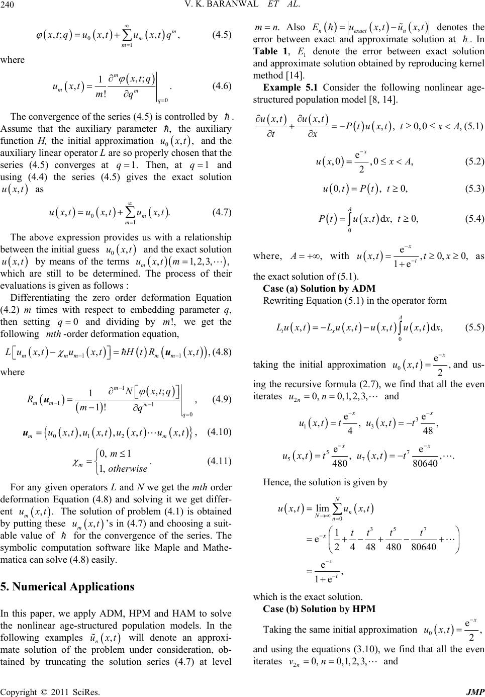

240 V. K. BARANWAL ET AL.
 
01
,;,, ,
m
m
m
x
tqu xtuxtq 



 (4.5)
where
 
0
,;
1
,!
m
mm
q
xtq
uxtmq



. (4.6)
The convergence of the series (4.5) is controlled by .
Assume that the auxiliary parameter the auxiliary
function H, the initial approximation and the
auxiliary linear operator L are so properly chosen that the
series (4.5) converges at

,
0
ux

,,t
1.q

Then, at 1q

and
using (4.4) the series (4.5) gives the exact solution
as

,uxt

,.

 
01
,,
m
m
uxtu xtuxt



 (4.7)
The above expression provides us with a relationship
between the initial guess and the exact solution
by means of the terms

0,uxt

,uxt




,1,2,3,
m
uxtm,
,,
which are still to be determined. The process of their
evaluations is given as follows :
Differentiating the zero order deformation Equation
(4.2) m times with respect to embedding parameter q,
then setting and dividing by we get the
following -order deformation eq uat i on,
0q
h!,m mt
  
11
,,
mmm mm
L uxtuxtH tRxt 



u(4.8)
where



1
11
0
,;
1
1!
m
mm m
q
Nxtq
Rmq






 u, (4.9)




012
,, ,,,,
mm
uxt u xt uxtuxtu


, (4.10)
0, 1
1,
m
m
otherwise




. (4.11)
For any given operators L and N we g et the mth order
deformation Equation (4.8) and solving it we get differ-
ent The solution of problem (4.1) is obtained
by putting these ’s in (4.7) and choosing a suit-
able value of for the convergence of the series. The
symbolic computation software like Maple and Mathe-
matica can solve (4.8) easily.

,.
m
uxt

,
m
uxt

5. Numerical Applications
In this paper, we apply ADM, HPM and HAM to solve
the nonlinear age-structured population models. In the
following examples will denote an approxi-
mate solution of the problem under consideration, ob-
tained by truncating the solution series (4.7) at level

,
n
uxt

.mn

Also


,
n exactn
Euxtux

,t denotes the
error between exact and approximate solution at . In
Table 1, 1 denote the error between exact solution
and approximate solution obtained by reproducing kernel
method [ 14] .

E
Example 5.1 Consider the following nonlinear age-
structured pop ul a ti on model [8, 14].



 
,, ,, 0,0 uxt Ptuxt tx
tx
 ,A
uxt (5.1)




e
,0 ,0,
2
x
uxx A


 (5.2)


0,, 0,utPtt

 (5.3)
 
0
,d, 0,
A
Ptuxtx t


 (5.4)
where, ,A

 with

e
,, 0,0,
d,
1e
x
t
uxtt x



 as
the exact solution of (5.1).
Case (a) Solution by ADM
Rewriting Equation (5.1) in the operator form

0
,,,,
A
tx
u xtLuxtu xtu xtx L (5.5)
taking the initial approximation

0e
,
x
,
2
uxt  and us-
ing the recursive formula (2.7), we find that all the even
iterates 20, 0,1,2,3,
n
un

 and
 
3
13
ee
,,,
44
x
,
8
x
uxt tuxtt


 
57
57
ee
,,, ,.
480 80640
xx
uxt tuxtt


Hence, the solution is given by
 
0
35 7
,lim ,
1
e2 4 48 48080640
e,
1e
N
n
Nn
x
x
t
uxtu xt
tt tt
 











which is the exact solution.
Case (b) Solution by HPM
Taking the same initial appro ximation

0e
2
,,
x
uxt  
and using the equations (3.10), we find that all the even
terates i20, 0,1,2,3,
n
vn

 and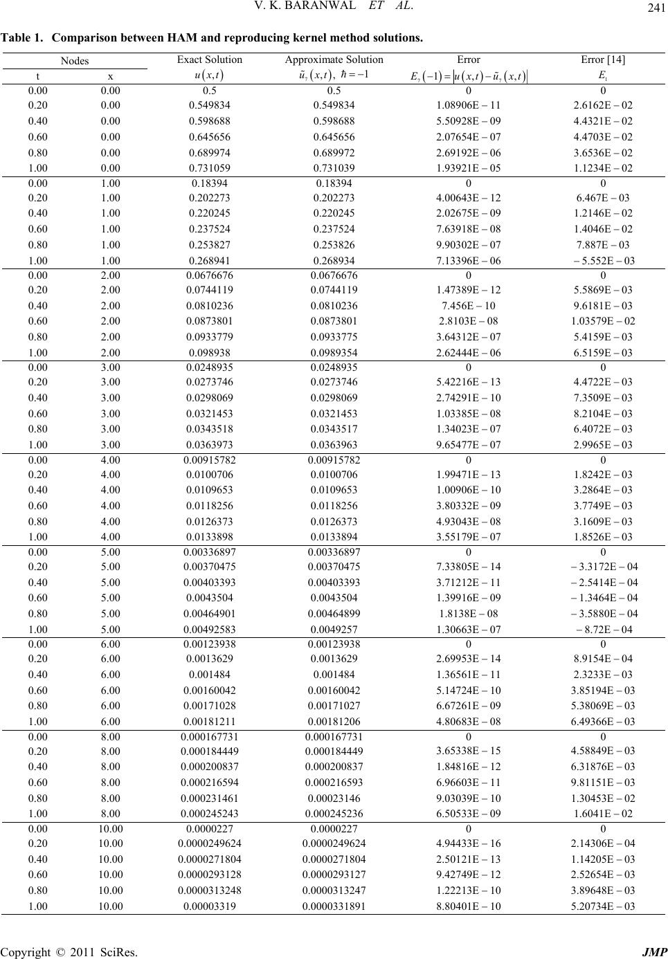

V. K. BARANWAL ET AL.
241
Table 1. Comparison between HAM and reproducing kernel method solutions.
Nodes
t x Exact Solution

,uxt Approximate Solution


7,,uxt
1

 Error
 
77
1, ,Euxtux  t Error [14]
1
E
0.00 0.00 0.5 0.5 0 0
0.20 0.00 0.549834 0.549834 1.08906E

11 2.6162E

02
0.40 0.00 0.598688 0.598688 5.50928E

09 4.4321E

02
0.60 0.00 0.645656 0.645656 2.07654E

07 4.4703E

02
0.80 0.00 0.689974 0.689972 2.69192E

06 3.6536E

02
1.00 0.00 0.731059 0.731039 1.93921E

05 1.1234E

02
0.00 1.00 0.18394 0.18394 0 0
0.20 1.00 0.202273 0.202273 4.00643E

12 6.467E

03
0.40 1.00 0.220245 0.220245 2.02675E

09 1.2146E

02
0.60 1.00 0.237524 0.237524 7.63918E

08 1.4046E

02
0.80 1.00 0.253827 0.253826 9.90302E

07 7.887E

03
1.00 1.00 0.268941 0.268934 7.13396E

06 5.552E

03
0.00 2.00 0.0676676 0.0676676 0 0
0.20 2.00 0.0744119 0.0744119 1.47389E

12 5.5869E

03
0.40 2.00 0.0810236 0.0810236 7.456E

10 9.6181E

03
0.60 2.00 0.0873801 0.0873801 2.8103E

08 1.03579E

02
0.80 2.00 0.0933779 0.0933775 3.64312E

07 5.4159E

03
1.00 2.00 0.098938 0.0989354 2.62444E

06 6.5159E

03
0.00 3.00 0.0248935 0.0248935 0 0
0.20 3.00 0.0273746 0.0273746 5.42216E

13 4.4722E

03
0.40 3.00 0.0298069 0.0298069 2.74291E

10 7.3509E

03
0.60 3.00 0.0321453 0.0321453 1.03385E

08 8.2104E

03
0.80 3.00 0.0343518 0.0343517 1.34023E

07 6.4072E

03
1.00 3.00 0.0363973 0.0363963 9.65477E

07 2.9965E

03
0.00 4.00 0.00915782 0.00915782 0 0
0.20 4.00 0.0100706 0.0100706 1.99471E

13 1.8242E

03
0.40 4.00 0.0109653 0.0109653 1.00906E

10 3.2864E

03
0.60 4.00 0.0118256 0.0118256 3.80332E

09 3.7749E

03
0.80 4.00 0.0126373 0.0126373 4.93043E

08 3.1609E

03
1.00 4.00 0.0133898 0.0133894 3.55179E

07 1.8526E

03
0.00 5.00 0.00336897 0.00336897 0 0
0.20 5.00 0.00370475 0.00370475 7.33805E

14 3.3172E

04
0.40 5.00 0.00403393 0.00403393 3.71212E

11 2.5414E

04
0.60 5.00 0.0043504 0.0043504 1.39916E

09 1.3464E

04
0.80 5.00 0.00464901 0.00464899 1.8138E

08 3.5880E

04
1.00 5.00 0.00492583 0.0049257 1.30663E

07 8.72E

04
0.00 6.00 0.00123938 0.00123938 0 0
0.20 6.00 0.0013629 0.0013629 2.69953E

14 8.9154E

04
0.40 6.00 0.001484 0.001484 1.36561E

11 2.3233E

03
0.60 6.00 0.00160042 0.00160042 5.14724E

10 3.85194E

03
0.80 6.00 0.00171028 0.00171027 6.67261E

09 5.38069E

03
1.00 6.00 0.00181211 0.00181206 4.80683E

08 6.49366E

03
0.00 8.00 0.000167731 0.000167731 0 0
0.20 8.00 0.000184449 0.000184449 3.65338E

15 4.58849E

03
0.40 8.00 0.000200837 0.000200837 1.84816E

12 6.31876E

03
0.60 8.00 0.000216594 0.000216593 6.96603E

11 9.81151E

03
0.80 8.00 0.000231461 0.00023146 9.03039E

10 1.30453E

02
1.00 8.00 0.000245243 0.000245236 6.50533E

09 1.6041E

02
0.00 10.00 0.0000227 0.0000227 0 0
0.20 10.00 0.0000249624 0.0000249624 4.94433E

16 2.14306E

04
0.40 10.00 0.0000271804 0.0000271804 2.50121E

13 1.14205E

03
0.60 10.00 0.0000293128 0.0000293127 9.42749E

12 2.52654E

03
0.80 10.00 0.0000313248 0.0000313247 1.22213E

10 3.89648E

03
1.00 10.00 0.00003319 0.0000331891 8.80401E

10 5.20734E

03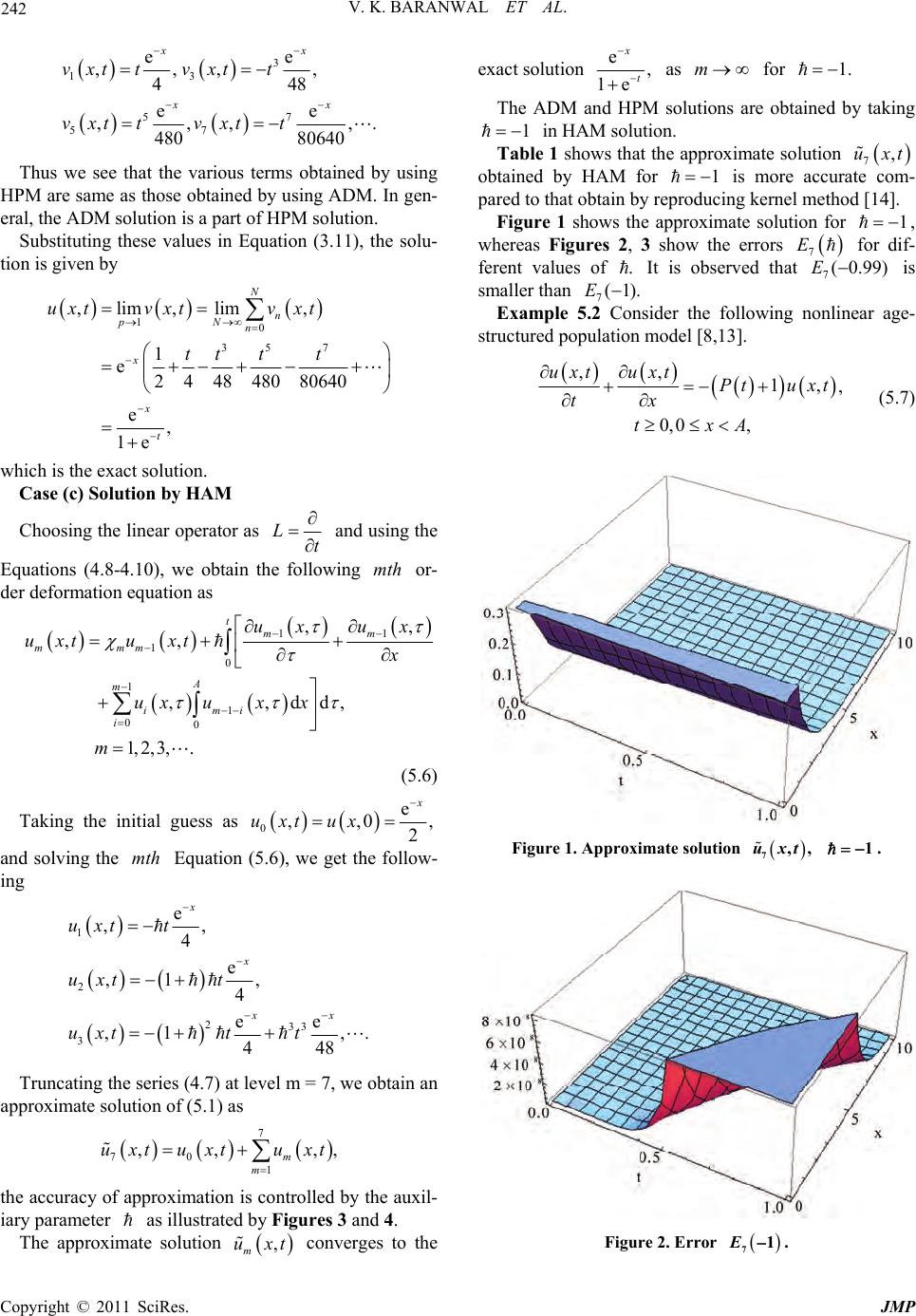

V. K. BARANWAL ET AL.
242
 
 
3
13
57
57
ee
,,, ,
448
ee
,,,
480 80640
xx
xx
vxt tvxtt
vxt tvxtt





, .
Thus we see that the various terms obtained by using
HPM are same as those obtained by using ADM. In gen-
eral, the ADM solution is a part of HPM solution.
Substituting these values in Equation (3.11), the solu-
tion is give n b y
 
10
35 7
,lim ,lim,
1
e244848080640
e,
1e
N
n
pN
n
x
x
t
uxtvxtvxt
tt tt













which is the exact solution.
Case (c) Solution by HAM
Choosing the linear operator as Lt

 and using the
Equations (4.8-4.10), we obtain the following or-
der deformation equation as mth
 


 
11
0
0
1
1
1
0
,,
,
1, 2, 3,
,,
,,dd
.
tmm
A
m
i
mmm
mi
i
uxux
x
u
uxt
x
u
x
t
m
ux
x





















(5.6)
Taking the initial guess as
 
0,,0
2
e,
x
uxtux 
and solving the Equation (5.6), we get the follow-
ing mth

 
 
1
2
233
3
e
,,
4
e
,1 ,
4
ee
,1 ,
448
x
x
xx
uxt t
uxt t
uxtt t





 


  .
, ,

Truncating the series (4.7) at level m = 7, we obtain an
approximate solution of (5.1) as
 
7
70 1
,,
m
m
uxtuxtuxt




the accuracy of approximation is controlled by the auxil-
iary parameter as illustrated by Figures 3 and 4. 
The approximate solution converges to the

,
m
uxt 
exact solution e,
1e
x
t


 as for m 1.
The ADM and HPM solutions are obtained by taking
1

 in HAM solution.
Table 1 shows th at the approximate solution


7,uxt

obtained by HAM for 1

 is more accurate com-
pared to that obtain by reproducing kernel method [14].
Figure 1 shows the approximate solution for 1


(0.99)
,
whereas Figures 2, 3 show the errors for dif-
ferent values of It is observed that

7
E
7
E . 

is
smaller than 7(1).E

Example 5.2 Consider the following nonlinear age-
structured po p ula t i on m odel [ 8, 13].






,, 1,
0,0 ,
uxtuxtPt uxt
tx
txA




,
(5.7)
Figure 1. Approximate solution

7,,

uxt 1

.
Figure 2. Error


71E.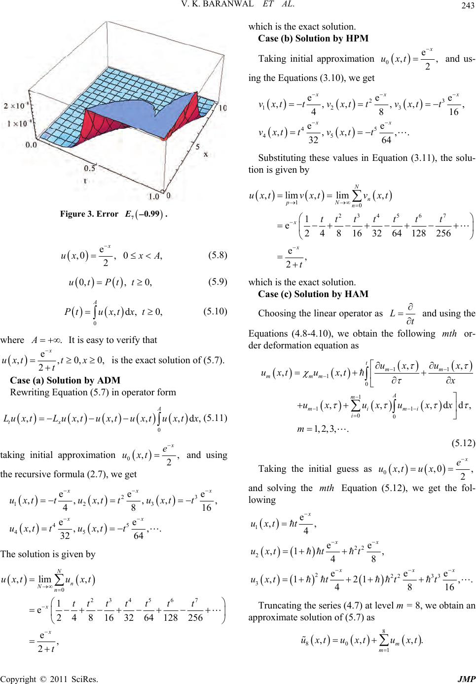

V. K. BARANWAL ET AL.
243
Figure 3. Error .

70.99E

e
,0,0,
2
x
uxxA


(5.8)
 
0,, 0,utPtt
(5.9)
 
0
,d, 0,
A
Ptuxtx t

(5.10)
where It is easy to verify that .A

e
,, 0,0,
2
x
uxtt x
t


 is the exact solution of (5.7).
Case (a) Solution by ADM
Rewriting Equation (5.7) in operator form

0
,,,,,
A
tx
Lu xtLu xtu xtu xtu xtx d, (5.11)
taking initial approximation

0,
2,
x
e
uxt   and using
the recursive formula (2.7), we get
  
 
2
123
45
45
ee
,,,,,
48
ee
,,,,.
32 64
3
e
,
16
x
x
xx
uxttuxttuxtt
uxttuxtt


 
 
x
The solution is given by
 
0
23 4 567
,lim ,
1
e248163264128256
e,
2
N
n
Nn
x
x
uxtu xt
tt ttttt
t
 




 






hich is the exact solution. wCase (b) Solution by HPM
Taking initial approximation

0e
,,
2
x
uxt   and us-
ing the Equat i o ns (3 .10), we get
  
 
23
123
45
45
ee e
,,,,, ,
48 16
ee
,,, ,.
32 64
x
xx
xx
vxttvxttvxtt
vxt tvxtt
 

 
 
Substituting these values in Equation (3.11), the solu-
tio

n is given by
 
10
23 4 567
,lim ,lim,
1
e2 4816 3264128 256
e,
2
N
n
pN
n
x
x
uxtvxtvxt
tt ttttt
t






 





which is the exact solution.
as
Case (c) Solution by HAM
Choosing the linear operator Lt

 and using the
Eqe follouations (4.8-4.10), we obtain thwing mth or-
der deformation equation as
 



11
0
1
11
00
1
,,
,,,d
.
,,
,
1, 2, 3,
d
mm
A
m
m
m
imi
i
mm
uxux
x
ux
uxtu xt
uu
m
xxx

t
























(5.12)
Taking the initial guess as
 
0,,0
2
x
e,uxt ux

an .12), we get the fold solving the mth Equation (5-
lowing

 
 
1
22
2
22233
3
e
,,
4
ee
,1 ,
48
ee
,1 21,
48
x
xx
xx
uxt t
uxtt t
uxttt t




 
 

 
 
e
.
16
x
Truncating the series (4.7) at level m = 8, we obtain an
ap
,.
proximate solution of (5.7) as
 
uxt uxt

8
80 1
,,
m
m
u xt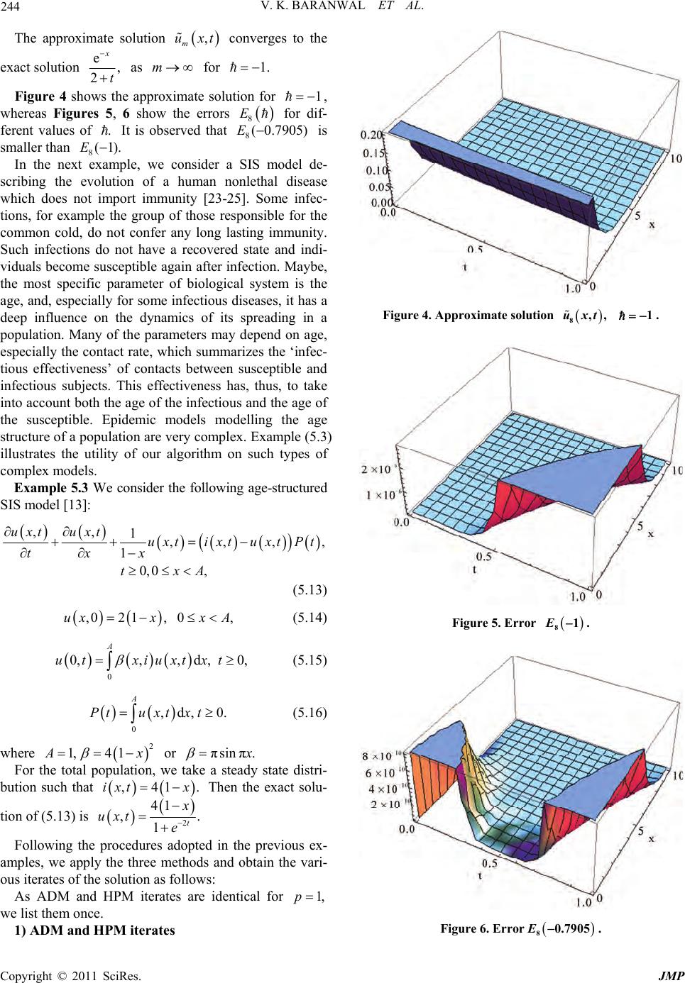




V. K. BARANWAL ET AL.
244
The approximate solution converges to the
exact solution

,
m
uxt

e,
2t
Figure 4 shows the approxlution for 1
x as m for
imate so
1.

,
or dif-
905) is
whereas Figur 6 show errors fes 5, the
fere
lunlethal dise

8
E
SIS m
nt values of . It is observed that 8( 0.7E
smaller than 8(1).E
In the next example, we consider a odel de-
scribing the evotion of a human noase
which does nort impot immunity [23-25]. Some infec-
tions, for example the group of those responsible for the
common cold, do not confer any long lasting immunity.
Such infections do not have a recovered state and indi-
viduals become su sceptible again after infection. Maybe,
the most specific parameter of biological system is the
age, and, especially for some infectious diseases, it has a
deep influence on the dynamics of its spreading in a
population. Many of the parameters may depend on age,
especially the contact rate, which summarizes the ‘infec-
tious effectiveness’ of contacts between susceptible and
infectious subjects. This effectiveness has, thus, to take
into account both the age of the infectious and the age of
the susceptible. Epidemic models modelling the age
structure of a popu lation are very complex. Example (5.3)
illustrates the utility of our algorithm on such types of
complex models.
Example 5.3 We consider the following age-structured
SIS model [13]:




  
,,
1,,,,
uxt uxtuxtixtuxtPt
tx

 
10,0 , x
txA



(5.13)
(5.14)

where
 
,02 1,0,uxxxA 
 
0
0,,,d ,
A
ut xiuxtxt  
0, (5.15)
 
0
,d, 0.
A
Ptuxt xt
 (5.16)

2
1,4 1
A
x   or πsin π.
x


take a stead y state distri-Fowe
ch that
r the total population,
bution su




,41ixt x .
Then the exact solu-
tion of (5.13) is
 
2
41
,.
t
1
x
uxt
Following the in the previous ex-
e 
procedures adopted
the three methods and obtain the vari-
ou

amples, we apply
s iterates of the solution as follows:
As ADM and HPM iterates are identical for 1,p

we list them once.
1) ADM and HPM iterates
Figure 4. Approximate solution

8,,

uxt 1

.


81E. Figure 5. Error
Figure 6. Error


80.7905E.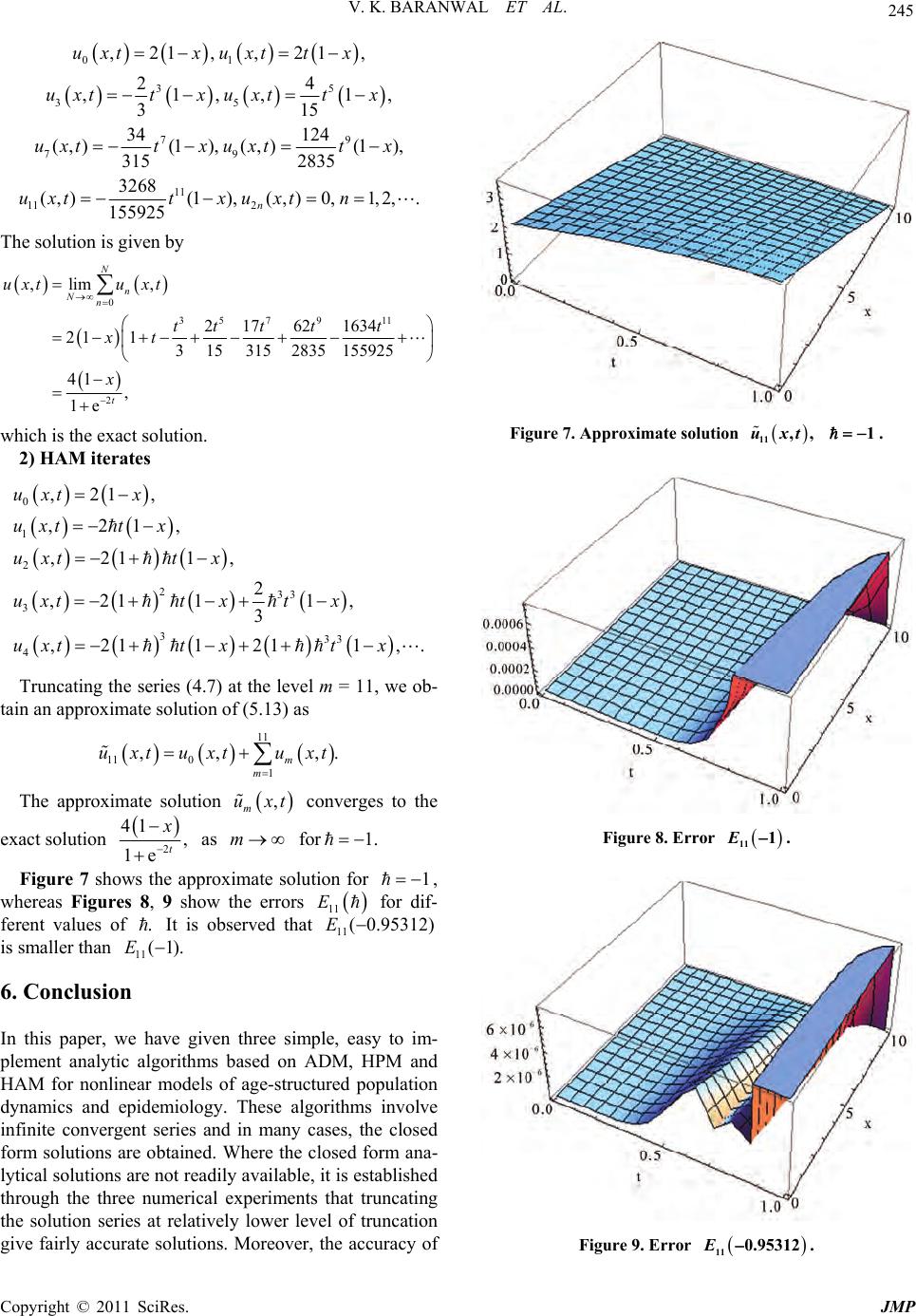

V. K. BARANWAL ET AL.
245
 


  
01
35
35
79
79
11
11 2
,21,,21,
24
,1,,1
315
34 124
(,)(1),(,)(1),
315 2835
3268
( ,)(1),( ,)0,1,2,.
155925 n
uxtxuxtt x
uxtt xuxtt x
uxtt xuxtt x
uxtt xuxtn
 
 
 
 
,
The solution is given by
 


0
35 7911
2
,lim ,
2 17621634
21 1 3153152835 155925
41 ,
1e
N
n
Nn
t
uxtu xt
tt ttt
xt
x
 



  






which is the exact solution.
2) HAM iterates



 
 
  
 
 
0
1
2
233
3
333
4
,21,
,21,
,21 1,
2
,21 11,
3
,211211,.
uxt x
uxtt x
uxttx
uxtt xtx
uxtt xtx

 
 

 


 
 
Truncating the series (4.7) at the level m = 11, we ob-
tain an approximate solution of (5.13) as
,.
The approximate solution converges to the
ex
 
11
11 01
,,
m
m
uxt uxtuxt





,
m
uxt

act solution

2
41 ,
t
1e
x


 as m fo
Figure 7 shows the approximate solution for
r1. 
1

,
for dif-
.95312)
whereas Figures 8, 9 show the errors
ferent values ofIt is observed th
is smaller than
6. Conclusion
In this paper, we have given three simple, easy to im-
pl
rithms involve
infinite convergent series and in many cases, the closed
form solutions are obtained. Where the closed form ana-
ly ailab
th xperime
ies at rel lowerl of trucation
give fairly accurate solutions. Moreover, the accuracy of

11
E
at 11( 0E
.
11
E (1).
ement analytic algorithms based on ADM, HPM and
HAM for nonlinear models of age-structured population
dynamics and epidemiology. These algo
tical solutions are not readily avle, it is established
rough the threenumerical ents that truncating
the solution seratively leven
Figure 7. Approximate solution


11 ,,

uxt 1

.
Figure 8. Error


11 1E.


11 0.95312E. Figure 9. Error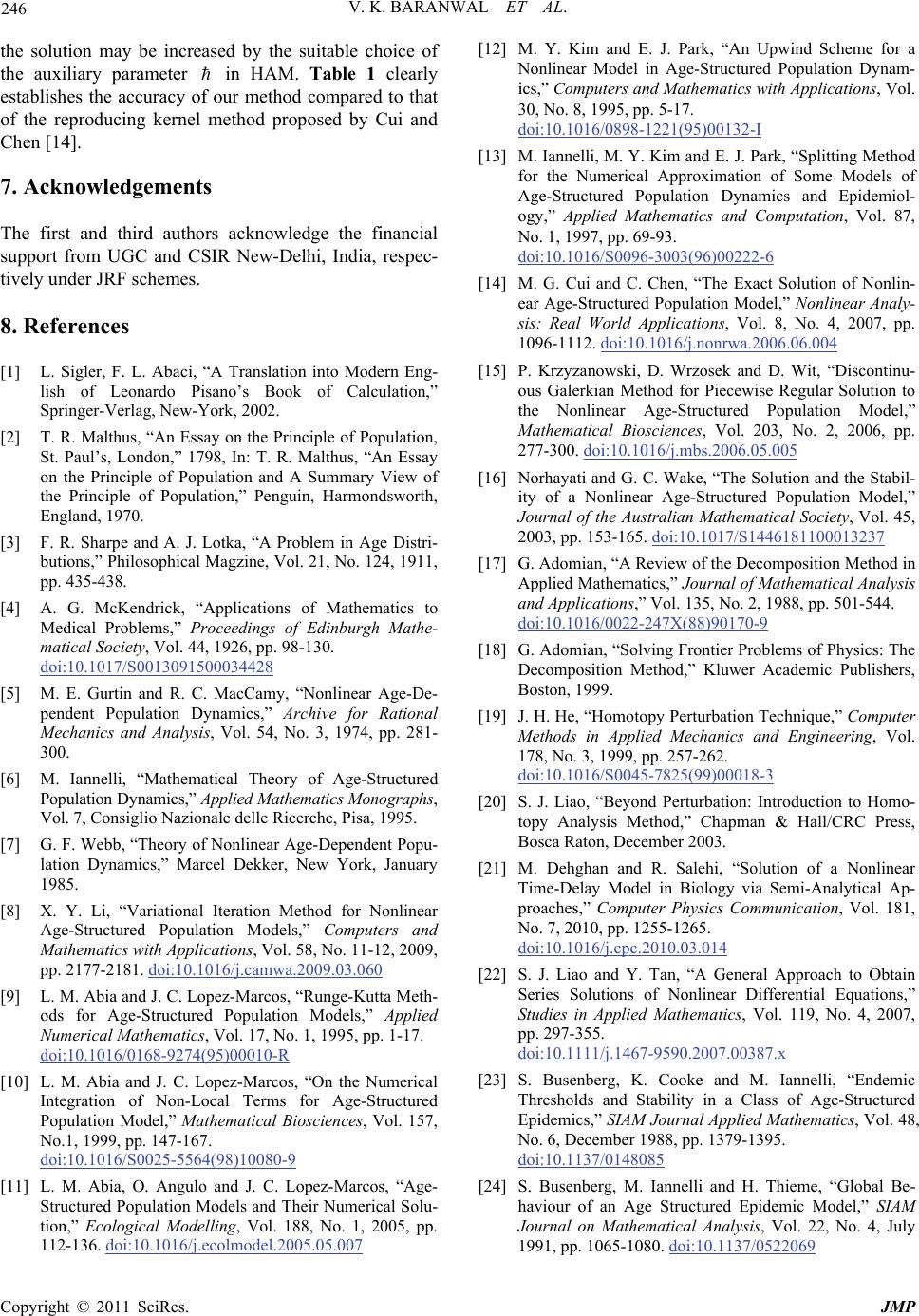

V. K. BARANWAL ET AL.
246
e solution may be increased by the suitable choice of
the auxiliary parameter in HAM. Table 1 clearly
establishes the accuracy of our method compared to that
of the reproducing kernel method proposed by Cui and
Chen [14].
7. Acknowledgements
The first and third authors acknowledge the financial
support from UGC and CSIR New-Delhi, India, respec
tively under JRF schemes.
8. References
[1] L. Sigler, F. L. Abaci, “A Translation into Modern
lish of Leonardo Pisano’s Book of Calculation,
Springer-Verlag, New-York, 2002.
[2] T. R. M the Principle of Population,
,” Philosophical Magzine, Vol. 21, No. 124, 1911,
lications of Mathematics to
th

-
Eng-
”
althus, “An Essay on
St. Paul’s, London,” 1798, In: T. R. Malthus, “An Essay
on the Principle of Population and A Summary View of
the Principle of Population,” Penguin, Harmondsworth,
England, 1970.
[3] F. R. Sharpe and A. J. Lotka, “A Problem in Age Distri-
butions
pp. 435-438.
4] A. G. McKendrick, “App[
Medical Problems,” Proceedings of Edinburgh Mathe-
matical Society, Vol. 44, 1926, pp. 98-130.
doi:10.1017/S0013091500034428
5] M. E. Gurtin and R. C. M[acCamy, “Nonlinear Ag
ynamics,” Archive for Rational
Analysis, Vol. 54, No. 3, 1974, pp. 281-
300.
cerche, Pisa, 1995.
Models,” Computers and
e-De-
pendent Population D
Mechanics and
[6] M. Iannelli, “Mathematical Theory of Age-Structured
Population Dynamic s,” Applied Mathematics Monographs,
Vol. 7, Consiglio Nazionale delle Ri
[7] G. F. Webb, “Theory of Nonlinear Age-Dependent Popu-
lation Dynamics,” Marcel Dekker, New York, January
1985.
[8] X. Y. Li, “Variational Iteration Method for Nonlinear
Age-Structured Population
Mathematics with Applications, Vol. 58, No. 11-12, 2009,
pp. 2177-2181. doi:10.1016/j.camwa.2009.03.060
[9] L. M. Abia and J. C. Lopez-Marcos, “Runge-Kutta Meth-
ods for Age-Structured Population Models,” Applied
Numerical Mathematics, Vol. 17, No. 1, 1995, pp. 1-17.
doi:10.1016/0168-9274(95)00010-R
[10] L. M. Abia and J. C. Lopez-Marcos, “On the Numerical
.1016/S0025-5564(98)10080-9
Integration of Non-Local Terms for Age-Structured
Population Model,” Mathematical Biosciences, Vol. 157,
No.1, 1999, pp. 147-167.
doi:10
p
[11] L. M. Abia, O. Angulo and J. C. Lopez-Marcos, “Age-
Structured Population Models and Their Numerical Solu-
tion,” Ecological Modelling, Vol. 188, No. 1, 2005, p.
112-136. doi:10.1016/j.ecolmodel.2005.05.007
[12] M. Y. Kim and E. J. Park, “An Upwind Scheme for a
Nonlinear Model in Age-Structured Population Dynam-
ics,” Computers and Mathematics with Applications, Vol.
30, No. 8, 1995, pp. 5-17.
doi:10.1016/0898-1221(95)00132-I
[13] M. Iannelli, M. Y. Kim and E. J. Park, “Splitting Method
for the Numerical Approximation of Some Models of
Age-Structured Population Dynamics and Epidemiol-
ogy,” Applied Mathematics and Computation, Vol. 87,
No. 1, 1997, pp. 69-93.
doi:10.1016/S0096-3003(96)00222-6
[14] M. G. Cui and C. Chen, “The Exact Solution of Nonlin-
ear Age-Structured Population Model,” Nonlinear Analy-
sis: Real World Applicati
1096-1112. ons, Vol. 8, No. 4, 2007, pp. .06.004doi:10.1016/j.nonrwa.2006
006, pp.
[15] P. Krzyzanowski, D. Wrzosek and D. Wit, “Discontinu-
ous Galerkian Method for Piecewise Regular Solution to
the Nonlinear Age-Structured Population Model,”
Mathematical Biosciences, Vol. 203, No. 2, 2
277-300. doi:10.1016/j.mbs.2006.05.005
[16] Norhayati and G. C. Wake, “The Solution and the Stabil-
ity of a Nonlinear Age-Structured Population Model,”
Journal of the Australian M
2003, pp. 153-165. athematical Society, Vol. 45, 6181100013237doi:10.1017/S144
[17] G. Adomian, “A Review of the Decomposition Method in
Applied Mathematics,” Journal of Mathematical Analysis
and Applications,” Vol. 135, No. 2, 1988, pp. 501-544.
doi:10.1016/0022-247X(88)90170-9
[18] G. Adomian, “Solving Frontier Problems of Ph
Decomposition Method,” Kluwer Acysics: The ademic Publishers,
Boston, 1999.
[19] J. H. He, “Homotopy Perturbation Technique,” Computer
Methods in Applied Mechanics and Engineering, Vol.
178, No. 3, 1999, pp. 257-262.
doi:10.1016/S0045-7825(99)00018-3
[20] S. J. Liao, “Beyond Perturbation: Introduction to Homo-
topy Analysis Method,” Chapman & Hall/CRC Press,
Bosca Raton, December 2003.
[21] M. Dehghan and R. Salehi, “Solution of a Nonlinear
Time-Delay Model in Biology via Semi-Analytical Ap-
proaches,” Computer Physics Communication, Vol. 181,
No. 7, 2010, pp. 1255-1265.
doi:10.1016/j.cpc.2010.03.014
[22] S. J. Liao and Y. Tan, “A General Approach to Obtain
Series Solutions of Nonlinear Differential Equations,”
Studies in Applied Mathematics, Vol. 119, No. 4, 2007
pp. 297-355. ,
doi:10.1111/j.1467-9590.2007.00387.x
[23] S. Busenberg, K. Cooke and M. Iannelli, “Endemic
Thresholds and Stability in a Class of Age-Structured
Epidemics,” SIAM Journal Applied Mathematics, Vol. 48,
No. 6, December 1988, pp. 1379-1395.
doi:10.1137/0148085
[24] S. Busenberg, M. Iannelli and H. Thieme, “Global Be-
haviour of an Age Structured Epidemic Model,” SIAM
Journal on Mathematical Analysis, Vol. 22, No. 4, July
1991, pp. 1065-1080. doi:10.1137/0522069

V. K. BARANWAL ET AL.
247
034
[25] M. Iannelli, F. Milner and A. Pugliese, “Analytical and
Numerical Results for the Age Structured SIS Epidemic
Model with Mixed Inter-Intracohort Transmission,”
SIAM Journal on Mathematical Analysis, Vol. 23, No. 3,
May 1992, pp. 662-688. doi:10.1137/0523