Journal of Modern Physics, 2011, 2, 219-224
doi:10.4236/jmp.2011.24030 Published Online April 2011 (http://www.SciRP.org/journal/jmp)
Quantization and Stable Attractors in a Dissipative
Orbital Motion
Daniel L. Nascimento, Antonio L. A. Fonseca
Institute of Physics and International Center for Condensed Matter, University of Brasília,
Brasília-DF, Brazil
Received October 15, 2010; revised December 27, 2010; accepted December 28, 2010
Abstract
We present a method for determining the motion of an electron in a hydrogen atom, which starts from a field
Lagrangean foundation for non-conservative systems that can exhibit chaotic behavior. As a consequence,
the problem of the formation of the atom becomes the problem of finding the possible stable orbital attractors
and the associated transition paths through which the electron mechanical energy varies continuously until a
stable energy state is reached.
Keywords: Stable Attractors, Non-Linear Dynamics, Non-Conservative Orbital Systems, Lagrangean
Systems, Electron Capture in Hydrogen Atom
1. Introduction
In this paper we present a new method for dealing with
quantization problems which is based, on the one hand,
on the concept of a stable attractor associated with a
non-linear differential equation from the usual chaos
theory and, on the other hand, on the variational formu-
lation of Quantum Mechanics introduced by E.
Schrödinger in 1926 [1]. That is, our approach is not
based in the current and well-known method of phase
space representation in the semi-classical limit of quan-
tum mechanics, usually known as “quantum chaos”.
The theory of quantum chaos was pioneered by Ein-
stein through his 1917 [2] paper, in which he made a
connection between classical and (old) quantum me-
chanics. This theory was further improved by many au-
thors, among which the works of Gutzwiller [3-7] and
Ozorio de Almeida [8-11] have made major contribu-
tions. In particular, Gutzwiller obtained in 1967 [3] the
exact wave functions for the bound states of the hydro-
gen atom, by performing a very complicated calculation
using a phase integral approximation of a Green’s func-
tion in momentum space.
We follow an alternative approach in this work, in
which we show that it is possible to obtain the exact en-
ergy of the bound states of the hydrogen atom by search-
ing for stable orbital attractors in a non-conservative
Hamilton-Jacobi dynamics [12-14]. Thus, the quantiza-
tion problem is solved by selecting, from all of the pos-
sible electron paths in which energy is dissipated, those
that tend to stable closed paths in which bound states of
motion are reached in the limit as time approaches infin-
ity, that is, to stable orbital attractors. This is done in
Section 2 where we are conducted from the well-known
linear Schrödinger equation to a non-linear momentum
equation. This equation will be shown to generate the
dissipative dynamics and allow the existence of a set of
stable attractors which prevent the collapse of the system.
In Section 3 we solve the equations for the hydrogen
atom obtaining the form of the dissipative energy func-
tion along the electron trajectory, in which the mechani-
cal energy varies continuously until a stable attractor is
reached, when it becomes finally constant.
2. The Equations of Motion
We start by considering the Hamiltonian function for an
electron which is considered as an ordinary charged par-
ticle, whose motion is caused by a scalar potential energy
function 2
Ve r and also that no vector potential is
present, i.e., 0

A. That is
2
2
H
V
m


p, (1)
where m

pv is the electron linear momentum,


1
p
mm m
ep e
mm

is the reduced mass and and
e
m

220 D. NASCIMENTO ET AL.
p
m are the electron and proton masses, respectively.
Of course, since in general the system irradiates con-
tinuously, the Hamiltonian (1) cannot be a constant of
the motion. Therefore, at first sight, the motion is always
dissipative, the electron tending to fall into the proton,
whose position may be called a collapsing attractor of the
process. Hence, we shall search in this work for the pos-
sibility of non-collapsing stable attractor paths toward
which the electron motion can tend asymptotically as
time goes to infinity.
Since is a spherically symmetric potential, this
implies the conservation of the angular momentum vec-
tor

Vr
r
L
p in the center of mass frame. Thus the mo-
tion should be plane, since r is always perpendicular to L,
from the initial moment until the stable motion is reached
in the limit as time goes to infinity. Because p and L are
mutually perpendicular vectors, and by using the linear
momentum radial and polar components r
pmr

 and
pmr


, respectively, and the relationships 0 L

rp

Lconstant and
H
E
constant, (1) assumes
the form
2
20
2
1
22
L
Emr V
mr

, (2)
which defines a conservative or Hamiltonian system in
Classical Mechanics.
It can immediately be seen that in this case (2) is a
non-linear equation in both and , so that Classical
Mechanics is in its deepest grounds a non-linear theory.
The closed paths that are solutions of Equation (2) are
elliptic orbits which may be obtained by integrating it
rr

directly, through the chain rule 0
2
d
d
L r
rmr


, as a func-
tion of the polar angle

. Alternatively we may also
observe that the only way that Equation (2) may be satis-
fied for any value of the continuous variable

is by a
composition of periodic sinusoidal functions of the form

11
1cos
ra


  , (3)
which substituted into Equation (2), and with the help of
the definition of the angular momentum, results respec-
tively in the following inverse average radius and eccen-
tricity formulae
2
0
2
2
,1
LaE
ame e  
2
(4)
A third way to address the Hamiltonian problem,
which is followed in usual Lagrangian Classical Me-
chanics, is to make use of a variational procedure to
transform the non-linear quadratic form given in (2) into
an ordinary linear second-order differential equation in
1r, whose solution is given exactly by the function in (3)
(see chap.2 of Ref. [15]). We shall follow a similar ap-
proach in this work.
It is a well known fact in Classical Mechanics that the
motion in any path corresponding to (3) is unstable
against energy loss by radiation, so that the electron in
fact follows a decreasing spiral motion toward the proton
position. In order to look for a stable orbital attractor,
that is, an orbit in which the motion can be stable against
a loss or gain of energy by emission or absorption of
radiation, we allow the Hamiltonian function in (1) to
vary along a virtual path and try to get a special state of
motion in which a loss in energy in a region of space
may be compensated by the absorption of energy in an-
other region, producing a self-restoration effect in the
Hamiltonian, so that, no net loss of energy occurs overall
and, therefore, the system becomes dynamically stable.
Thus, we consider along the path given by the classi-
cal linear momentum p, which is the solution of (1) with
H
E

, linear momentum variation vectors


pp
,
which vary to the left or to the right of p by , which is
a solution of Equation (1) if
p
H
E. This variation
momentum must satisfy the asymptotic limit , as
, that define the stable attractors which we are
looking for. At this limit, we get back to the p path at a
matching point
0p
t
a
rr

, but with specific values for the
parameters and 0 which determine the specific
ellipses that make the system stable or self-restoring.
EL
In order to accomplish this, we shall observe that, due
to the emission of radiation, the finite difference
 
222mH E pp pppp (5)
must approach zero if
H
E as t. Also, in the
absorption process, Equation (5) must approach zero if

H
E

as . In any case, (5) must be expressed
as a quadratic form which is suitable for the variational
procedure. This is made by introducing a variation func-
tion
t


r   through a transformation proposed
originally by Schrödinger [1]:


 p

, (6)
where is the rationalized Planck’s constant.

The Lagrangian density function we need is then ob-
tained by considering 2

times the difference between
the Hamiltonian H and the energy attractor E. After sub-
stituting (6) into (5) and using (1) we obtain
 
2
22 2QHE mVE 2
 
 . (7)
Here,


,,QQ r  
is a quadratic form of the
function

and its space derivatives, so that the varia-
tion of the volume integral of Q conducts to a partial
linear differential equation, as expected in a Lagrange’s
variational problem.

D. NASCIMENTO ET AL.
221
We also need to impose the constraint that the function

must be square integrable or normalizable, because
2

stands for an averaging weight function
2d
space
V  1

, (8)
where, for simplicity, the unity value for the normaliza-
tion constant has been assumed.
Let us consider now the calculation of the volume in-
tegral d
space
I
QV over all space. If there is a finite
loss or gain of energy due to radiation,
H
E is a fi-
nite quantity too. In order to avoid collapse of the system
I must be a finite constant. In order to assure that, it is
enough that Q is limited at the origin and tend to zero as
the space volume tends to infinity. Therefore, in order to
allow the existence of stable attractors, we shall impose
that I must have an extreme value near zero1 so that its
variation vanishes, namely
d
space
QV0

. (9)
It will be seen in what follows that only trajectories
which tend to a closed path as time goes to infinity will
satisfy the variational problem, reaching a stable attractor
path. Equation (9) cannot be satisfied if we consider ei-
ther the free electron motion or the motion in a scattering
process, since such motions are remarkably unbound,
and therefore cannot satisfy (8).
Now, by introducing the Lagrangian density, (7), into
(9), we get

2
2
d
2
+d
2
space
surface
EV V
m
m





 


0





F
. (10)
In the calculation of the variations, usual integration
by parts has been made and d
F
is the surface element
vector. In order to satisfy (10), it is sufficient to require
that the integrand in the volume integral and the surface
integral vanish separately, namely

22mEV
  0 
0
(11)
and
d
surface
  
F. (12)
Equation (11) is the variational form of the Schrödinger
equation and (12) is automatically satisfied by the re-
quirement that the variation


vanishes at infinity,
where the surface integral is calculated, although it
would also be asked to vanish on a finite surface2. This is
guaranteed by the constraint (8), which implies that

as well as


vanish at infinity.
Now, from (11), we can obtain an equation for the var-
ied linear momentum of the electron through (6) and the
identity
2


  


 
 
 
0
, (13)
which substituted into Equation (11) results in
 
22mE V

 pp . (14)
From this non-linear momentum variation equation for
a non-conservative system, which is analogous to (2) for
a conservative system, the electron trajectories resulting
in the stable attractor mentioned above will be obtained.
Thus, Equation (11) is the linear differential equation
associated with the non-linear momentum equation, (14).
3. Determination of the Electron Path
Functions in the Formation of a
Hydrogen Atom
We can now perform the reduction of both the equations
of motion, (11) and (14). Starting with the former, we
consider a variation in path with a constant angular mo-
mentum3 0 L

 , so that . This value assigned
to L is provisory because the actual value will come from
the specific orbits to be found. Thus,
0L


r  depends
only on the radius and hence (11) becomes
222
22 2
d 20
d
d
me
E
rr r
rr
 


d1


 





, (15)
where the numeric factor will be determined later. 
The radial variation may be obtained through (6) as
d
d
r
pr


. (16)
Now, we remember that the divergence of a vector u
in polar coordinates is
2
11
r
r
u
uu
rr r




 


u, (17)
through which we can reduce (14) to its radial form,
namely



22 2
2
2
d20
d
rr
r
ppe
pmE
rr r
r



 
 
  

 ,
(18)

2This will be considered in a future work concerning discrete transitions.
3We will consider a variable angular momentum in a future work in
connection with the transition between energy levels.
1It would be exactly zero for a Hamiltonian system, since in this case H =
E
always.

222 D. NASCIMENTO ET AL.
where is the above-mentioned parameter.

Since (18) is non-linear, it is not a simple task to ob-
tain its solution directly. Instead of this, we shall employ
the radial solutions of the linear (15), and generate solu-
tions for the (18), through (16). In its simplest form the
solutions for (15) that are regular at the origin and at in-
finity can be written as [16]

0
rr
Rr re



, (19)
which, after substitution into (15) and equating coeffi-
cients in the same power, yields
B
2
E
1
2
E





, (20)
where
22
213.6 eV
22
B
BB
e
Eama  
 is the ionization or
Bohr energy of the hydrogen atom. We see immediately
that the only possible values for the parameter which
make the above expression for the energy levels to agree
with the experiment are the half-integers4:

135
,,,
222

Thus, the solution of (18) obtained through (19) be-
comes
0
11
r
prr 


 
  . (21)
Therefore the simplest stable attractor condition is
given by and the possible stable attractor
radii are given by

00 r
pr

0
1
2
B
r




 a, (22)
where
2
20.53
B
ame 
Å, is the Bohr radius. The plot
of Equation (21) for 135 ,,
222
 is shown in Figure 1,
in which 0 assumes the values 0.5, 3.0 and 7.5 a.u.,
respectively. We note that for 0, we have
r
rr0
r
p

so that the three curves correspond to decreasing spirals
toward 0. On the other hand, for 0, we have
, so that the three curves correspond to increasing
spirals also toward 0, therefore illustrating the work-
ings of the self-restoring effect. Thus 0 is really an
asymptotically stable orbital point, i.e. a stable attractor.
rrr
r
0
r
p
r
By considering now the solution (21) of the non-linear
equation (18) and again comparing coefficients in the
same power, we obtain the same energy levels specified
by (20). And from the radii given in (22) we can calcu
Figure 1. The radial varied linear momenta


r
p
r, where
r is in a.u., for 1
2


(solid line), 3
2
 (dashed line) and
5
2


(dotted line).
late the values of the derivative of the variation of the
radial component of the linear momentum


2
d
d
o
r
o
r
p
rr


 , (23)
which, once inserted into Equation (18), yields the con-
servative form
 
2
2
12
o
o
Vr E
mr





 . (24)
We see that, for


00 r
pr

 and with

01L


 , (24) has the same classical con-
servation form as (2), which is consequently the actual
value of the angular momentum. Therefore, the resulting
conservative orbit is described in phase space by the
twofold function

2
2
2
1
2
r
e
pmE
rr


 



 . (25)
The plot of (25) together with the radial variation (21)
are shown in Figure 2 for 1
2
, from which we can
note that 0 (= 0.5 a.u.) is the intersection point of the
paths because it is their only common root.
r
In addition, is not the only root of (24) or for the
condition 0
r
0
r
p

in (25); the other root being

0
1
12
B
r




a
, (26)
so that 0 and 0
r r

 become respectively the semiminor
and semimajor axes of the ellipse
4These half-integers will be connected with periodic wave conditions in a
future work.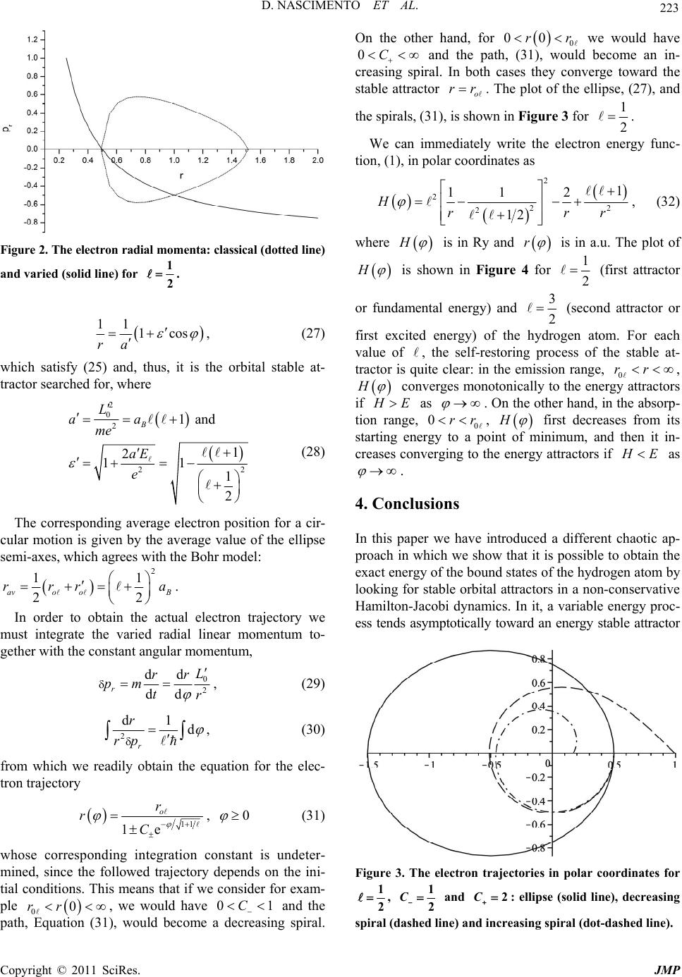

D. NASCIMENTO ET AL.
223
Figure 2. The electron radial momenta: classical (dotted line)
and varied (solid line) for 1
2
.

11
1cos
ra


 
, (27)
which satisfy (25) and, thus, it is the orbital stable at-
tractor searched for, where


2
0
2
22
1 and
1
2
11
1
2
B
L
aa
me
aE
e


 


 








(28)
The corresponding average electron position for a cir-
cular motion is given by the average value of the ellipse
semi-axes, which agrees with the Bohr model:

2
11
22
avo oB
rrr





 a.
In order to obtain the actual electron trajectory we
must integrate the varied radial linear momentum to-
gether with the constant angular momentum,
0
2
dd
dd
r
L rr
pm
tr 
  , (29)
2
d1
d
r
r
rp




, (30)
from which we readily obtain the equation for the elec-
tron trajectory

11
1e
o
r
r
C






, 0


1
r
(31)
whose corresponding integration constant is undeter-
mined, since the followed trajectory depends on the ini-
tial conditions. This means that if we consider for exam-
ple , we would have and the
path, Equation (31), would become a decreasing spiral.
On the other hand, for we would have

00rr 0C


0
00r

0C

 and the path, (31), would become an in-
creasing spiral. In both cases they converge toward the
stable attractor o rr

. The plot of the ellipse, (27), and
the spirals, (31), is shown in Figure 3 for 1
2
.
We can immediately write the electron energy func-
tion, (1), in polar coordinates as
 

2
2
2
2
1
11 2
12 2
rr r


  
 




H  , (32)
where


H

is in Ry and

r

is in a.u. The plot of


H

is shown in Figure 4 for 1
2
 (first attractor
or fundamental energy) and 3
2
 (second attractor or
first excited energy) of the hydrogen atom. For each
value of , the self-restoring process of the stable at-
tractor is quite clear: in the emission range, 0

rr


,


H

converges monotonically to the energy attractors
if
H
E as


rr
. On the other hand, in the absorp-
tion range, 0
0

,


H

first decreases from its
starting energy to a point of minimum, and then it in-
creases converging to the energy attractors if
H
E

as

.
4. Conclusions
In this paper we have introduced a different chaotic ap-
proach in which we show that it is possible to obtain the
exact energy of the bound states of the hydrogen atom by
looking for stable orbital attractors in a non-conservative
Hamilton-Jacobi dynamics. In it, a variable energy proc-
ess tends asymptotically toward an energy stable attractor
Figure 3. The electron trajectories in polar coordinates for
1
2


, 1
2
C

and 2C

: ellipse (solid line), decreasing
spiral (dashed line) and increasing spiral (dot-dashed line).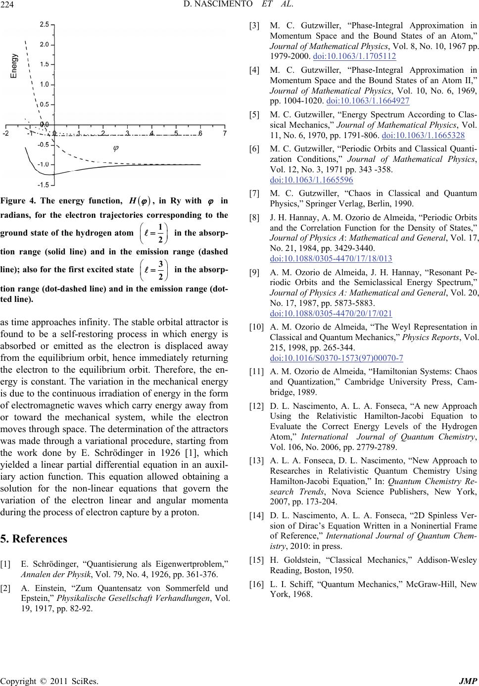

D. NASCIMENTO ET AL.
224
[3] M. C. Gutzwiller, “Phase-Integral Approximation in
Momentum Space and the Bound States of an Atom,”
Journal of Mathematical Physics, Vol. 8, No. 10, 1967 pp.
1979-2000. doi:10.1063/1.1705112
[4] M. C. Gutzwiller, “Phase-Integral Approximation in
Momentum Space and the Bound States of an Atom II,”
Journal of Mathematical Physics, Vol. 10, No. 6, 1969,
pp. 1004-1020. doi:10.1063/1.1664927
[5] M. C. Gutzwiller, “Energy Spectrum According to Clas-
sical Mechanics,” Journal of Mathematical Physics, Vol.
11, No. 6, 1970, pp. 1791-806. doi:10.1063/1.1665328
[6] M. C. Gutzwiller, “Periodic Orbits and Classical Quanti-
zation Conditions,” Journal of Mathematical Physics,
Vol. 12, No. 3, 1971 pp. 343 -358.
doi:10.1063/1.1665596
[7] M. C. Gutzwiller, “Chaos in Classical and Quantum
Physics,” Springer Verlag, Berlin, 1990.
Figure 4. The energy function,


H, in Ry with

in
radians, for the electron trajectories corresponding to the
ground state of the hydrogen atom 


[8] J. H. Hannay, A. M. Ozorio de Almeida, “Periodic Orbits
and the Correlation Function for the Density of States,”
Journal of Physics A: Mathematical and General, Vol. 17,
No. 21, 1984, pp. 3429-3440.
doi:10.1088/0305-4470/17/18/013



1
2 in the absorp-
tion range (solid line) and in the emission range (dashed
line); also for the first excited state 




3
2 in the absorp-
tion range (dot-dashed line) and in the emission range (dot-
ted line).
[9] A. M. Ozorio de Almeida, J. H. Hannay, “Resonant Pe-
riodic Orbits and the Semiclassical Energy Spectrum,”
Journal of Physics A: Mathematical and General, Vol. 20,
No. 17, 1987, pp. 5873-5883.
doi:10.1088/0305-4470/20/17/021
as time approaches infinity. The stable orbital attractor is
found to be a self-restoring process in which energy is
absorbed or emitted as the electron is displaced away
from the equilibrium orbit, hence immediately returning
the electron to the equilibrium orbit. Therefore, the en-
ergy is constant. The variation in the mechanical energy
is due to the continuous irradiation of energy in the form
of electromagnetic waves which carry energy away from
or toward the mechanical system, while the electron
moves through space. The determination of the attractors
was made through a variational procedure, starting from
the work done by E. Schrödinger in 1926 [1], which
yielded a linear partial differential equation in an auxil-
iary action function. This equation allowed obtaining a
solution for the non-linear equations that govern the
variation of the electron linear and angular momenta
during the process of electron capture by a proton.
[10] A. M. Ozorio de Almeida, “The Weyl Representation in
Classical and Quantum Mechanics,” Physics Reports, Vol.
215, 1998, pp. 265-344.
doi:10.1016/S0370-1573(97)00070-7
[11] A. M. Ozorio de Almeida, “Hamiltonian Systems: Chaos
and Quantization,” Cambridge University Press, Cam-
bridge, 1989.
[12] D. L. Nascimento, A. L. A. Fonseca, “A new Approach
Using the Relativistic Hamilton-Jacobi Equation to
Evaluate the Correct Energy Levels of the Hydrogen
Atom,” International Journal of Quantum Chemistry,
Vol. 106, No. 2006, pp. 2779-2789.
[13] A. L. A. Fonseca, D. L. Nascimento, “New Approach to
Researches in Relativistic Quantum Chemistry Using
Hamilton-Jacobi Equation,” In: Quantum Chemistry Re-
search Trends, Nova Science Publishers, New York,
2007, pp. 173-204.
[14] D. L. Nascimento, A. L. A. Fonseca, “2D Spinless Ver-
sion of Dirac’s Equation Written in a Noninertial Frame
of Reference,” International Journal of Quantum Chem-
istry, 2010: in press.
5. References
[15] H. Goldstein, “Classical Mechanics,” Addison-Wesley
Reading, Boston, 1950.
[1] E. Schrödinger, “Quantisierung als Eigenwertproblem,”
Annalen der Physik, Vol. 79, No. 4, 1926, pp. 361-376.
[16] L. I. Schiff, “Quantum Mechanics,” McGraw-Hill, New
York, 1968.
[2] A. Einstein, “Zum Quantensatz von Sommerfeld und
Epstein,” Physikalische Gesellschaft Verhandlungen, Vol.
19, 1917, pp. 82-92.
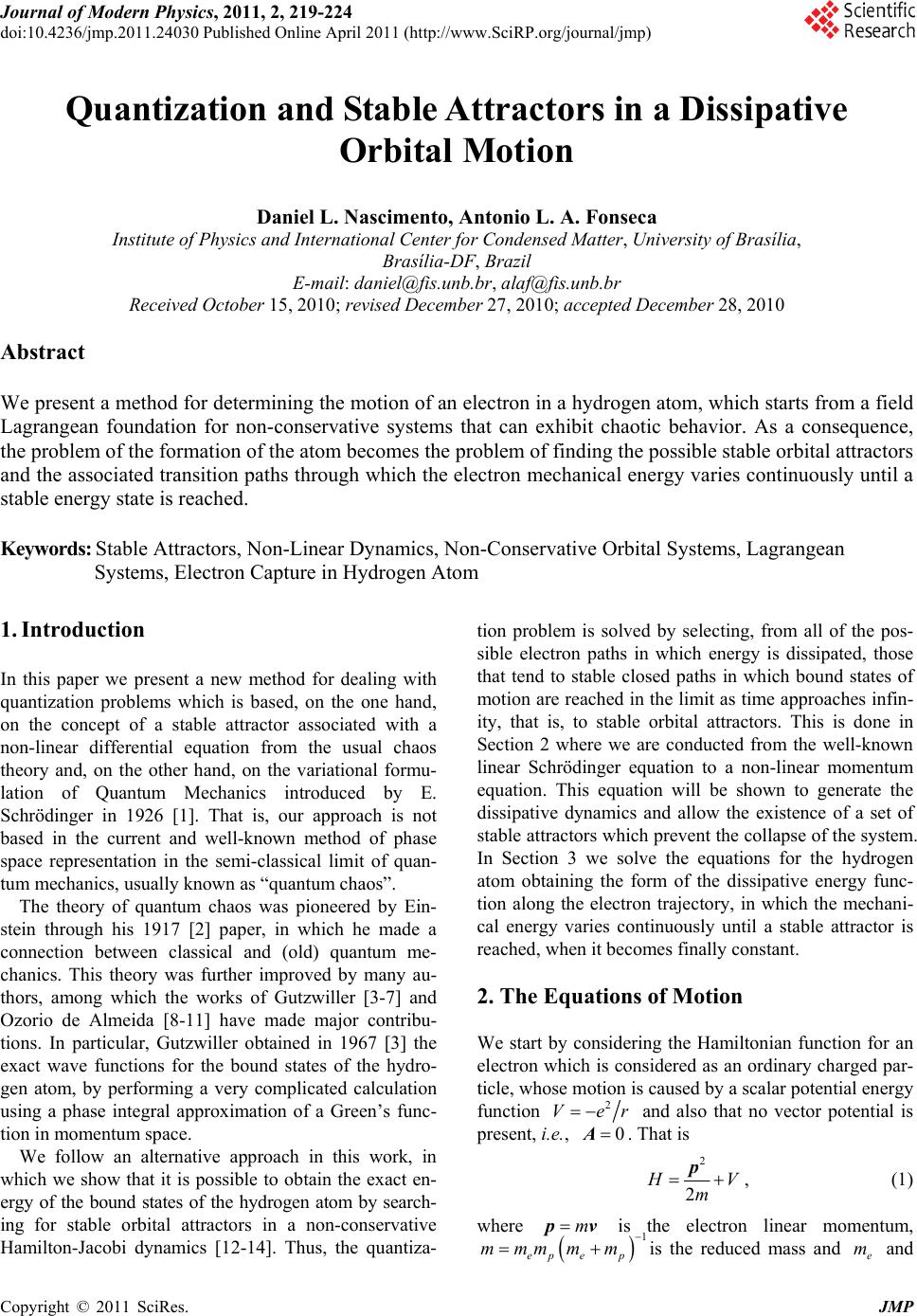