Vol.3, No.4, 301-306 (2011) Natural Science
http://dx.doi.org/10.4236/ns.2011.34039
A new improved filter for target tracking: compressed
iterative particle filter
Hongbo Zhu1*, Hai Zhao2, Dan Liu2, Chunhe Song2
1Software College Northeastern University, Shenyang, China; *Corresponding Author:
2Institute of Information and Technology Northeastern University, Shenyang, China;
Received 27 October 2010; revised 25 November 2010; accepted 20 December 2010.
ABSTRACT
Target tracking in video is a hot topic in com-
puter vision field, which has wide applications
in surveillance, robot navigation and human-
machine interaction etc. Meanshift is widely
used algorithm in video target tracking field.
The basic mean shift algorithm only considers
the color of targets as the tracking characteris-
tic feature, so if the appearance of the target
changes greatly or there exits other objects
whose color is similar to the target, the tracking
process will fail. To enhance the stability and
robustness of the algorithm, we introduce par-
ticle filter into the tracking process. Basic parti-
cle filter has some disadvantages such as low
accuracy, high computational complexity. In this
paper, an improved particle filter GA-UPF was
proposed, in which a new re-sampling algorithm
was used to predict target centroid position.
The target tracking system of binocular stereo
vision is designed and implemented. Experi-
mental results have shown that our algorithm
can tracking object in video with high accuracy
and low computational complexity.
Keywords: Filtering Method; Particle Filtering;
Unscented Particle Filter; Genetic Algorithm;
Target Tracking
1. INTRODUCTION
Target tracking in video is a hot topic in computer vi-
sion field, which has wide applications in surveillance,
robot navigation and human-machine interaction etc.
Many algorithms are proposed, but if the appearance of
the target changes greatly or there exits other objects
who are affected by the occasion. To enhance the stabil-
ity and robustness of the algorithm, particle filter is in-
troduced into the tracking process. Basic particle filter
(PF) has some disadvantages such as low accuracy, high
computational complexity. Due to solve the problem, an
improved particle filter GA-UPF was proposed.
GA-UPF is the integration of genetic algorithm (GA)
and unscented particle filter (UPF). It successfully off-
sets the defect in PF. And GA makes sure that particle
degeneracy phenomenon and particle sample impove-
rishment in re-sample process cannot be discovered.
Experimental results have shown that our algorithm has
better filtering effect.
The remaining of the paper is organized as follows: in
the Section 2, a brief description of GPF is presented. In
the Section 3, firstly, the GA algorithm is introduced,
and a new type GA – one-step predefined GA process is
proposed. Then the details of the new PF this paper pro-
posed – GA-UPF is presented. In Section 4 the proposed
algorithm is compared to other several different filtering
algorithms, and finally, some concluding remarks is
given in Section 5.
2. BASIC PARTICLE FILTER
The system probability model set as

1tt
pxx
 and


tt
pyx , and the system follows the Markov process.
The problem being addressed here is an estimating
problem of the state of a system as a set of observations
becomes available on-line. The initial value of prior
probability density function is

0
px . The complete
solution of sequential estimation problem is the poste-
riori probability density function

0: 1:tt
px y.
Using Monte Carlo sampling points, particle filter
executes the filtering process by generating weighted
sampling points of state variances recursively. A group of
random testing value is
 

 0: ,
ii
tt
xw ,

 0: , 1,,
i
k
x
iN
is sample set. As the corresponding weights,



, 1,,
i
t
wi N content with 1
i
t
iw
. The poste-
riori probability density function is similar as:


 

0:
0: 1:0:
1δ
t
Ni
i
ttk t
i
px ywxx


 (1)

H. B. Zhu et al. / Natural Science 3 (2011) 301-306 302
Through introducing and resampling the key density

0: 1:tt
qx y, the result is as follow:


0: 0: 1: t
i
tt
x
qx y (2)
As Bayes theory and re-sampling principle, the condi-
tion of [1]:





0:
0:
1:
1:
t
t
i
t
i
ti
t
px y
w
qx y
 (3)
Setting decomposition of the key density:

0:1:0: 11:0: 11: 1
,
tttttt t
qx yqxxy qxy

 (4)
Generic particle filter algorithm can be predicted as
follows [2]:
Initialization
For each particle
Draw the states

0
i
x
from the prior

0
px ;
End
For each loop
Importance sampling step
For each particle
Sample
 
 00:11:
ˆ~,
ii
tt t
x
qxxy

End
For each particle
Evaluate the importance weights up to a normalizing
constant:
 
 

 

1
1
0: 11:
ˆ
()
ˆˆ,
iii
tttt
ii
tt ii
tt t
py xpxx
ww
qx xy



 (5)
For each particle, normalize the importance weights:
 
1
1
1
N
ii j
tt t
j
ww w






 (6)
//Re-sample
Eliminate the samples with low importance weights
and multiply the samples with high importance weights,
to obtain N random samples

0:
i
k
x
approximately distri-
buted according to

0: 1:kk
px z.
Assign each particle an equal weight: 1
i
t
wN. When
executing particle filtering, the choice of the proposal
distribution is very important. Usually, the transition
prior distribution is chosen to be the proposal distribu-
tion:

11
,
tt ttk
qxX Ypxx

 (7)
But as not considering the recent observation, when
using the transition prior distribution as the proposal
distribution, the filtering result is usually poor, especially
when the noise is heavy. In this paper, a kind of semi-
iterative unscented transformation was proposed to ad-
dress this issue.
3. THE GENETIC ALGORITHM
3.1. Genetic Algorithm
GA is an optimization strategy generally employed to
find a global best point. In a genetic algorithm, a popula-
tion of strings (called chromosomes or the genotype of
the genome), which encode candidate solutions (called
individuals, creatures, or phenotypes) to an optimization
problem, evolves toward better solutions. There are three
main steps in the whole GA process, which consists of
Selection, Crossover and Mutation as Figure 1.
GA is a search heuristic that mimics the process of
natural evolution. This heuristic is routinely used to
generate useful solutions to optimization and search
problems as Figure 1. Using pseudo code to descript the
simple generational genetic algorithm is as follow:
1) The initial population of individual must be chosen.
2) Evaluate the fitness of each individual in that popu-
Figure 1. Process of genetic algorithm (GA).

H. B. Zhu et al. / Natural Science 3 (2011) 301-306 303
lation.
3) Make selection of the best-fit individuals for re-
production.
4) Breed new individuals through crossover and
mutation operations to give birth to offspring.
5) Evaluate the individual fitness of new individuals.
6) Replace least-fit population with new individuals.
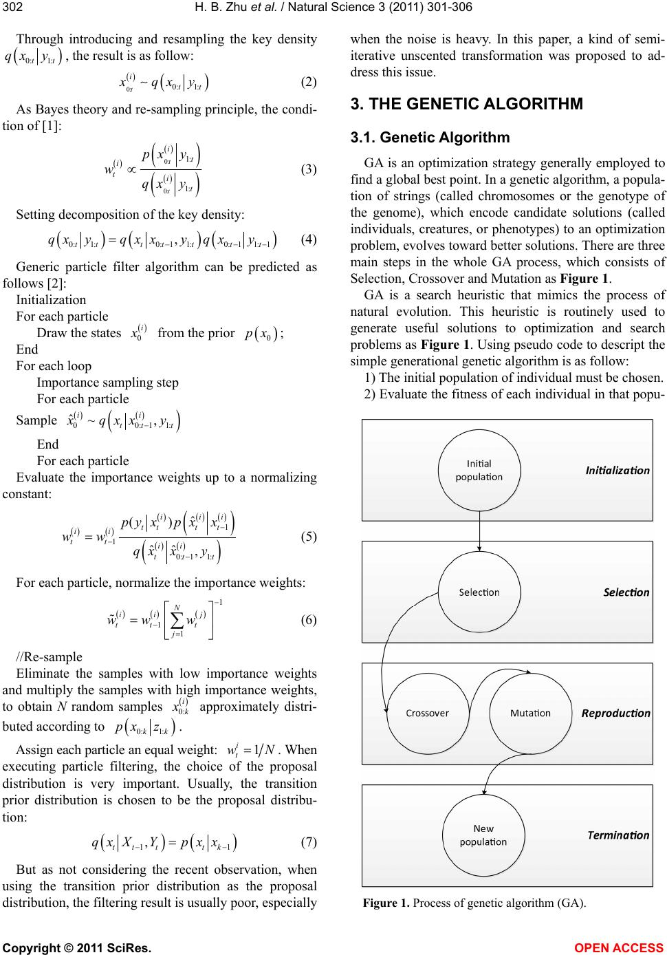
3.2. GA in the PF Process
The particles degeneration phenomenon is a wide-
spread problem of particle filter algorithm. In order to
eliminate that phenomenon, the re-sample algorithm is
introduced as depicted in the Section 2. In the re-sam-
pling process of regular particle filtering, the particles
with bigger weights will have more offspring, while the
particles with smaller weights will have few or even on
offspring. It inspires us to reduce the number of particles
with small weights and find more particles with big
weights, which will make the proposal distribution more
closed to the poster distribution. But re-sampling algo-
rithm causes another problem which loses particle diver-
sity and reduces the performance of the particle filter
algorithm, and even makes the distribution function of
particle filter algorithm spread. Therefore GA is pro-
posed in PF process.
The choice of fitness function is the most important
issue of using genetic algorithm. In the proposed algo-
rithm, each particle in particle algorithm is looked upon
a pair of chromosome. We want to find more particles
with bigger weights, so the fitness can be chosen as the
value of weights directly. As usually the aim of GA al-
gorithms is to minimize the fitness function, so the fit-
ness is the minus value of particle weight in the GA-PF
as follows:



 

 

1
0: 11:
ˆ
ˆˆ ,
iii
ttt t
i
tii
tt t
pyxpxx
fitness
qx xy


 (8)
Secondly, it’s already so large to compute consump-
tion of particle filtering that the GA process computing
consumption introduced should be reduced. In the
GA-PF algorithm, for every particle, at first, a random
number in the range of 0 and 1 will be generated, and
only when the number is smaller than a predefined
threshold, the GA process can be conducted. A new type
of GA process – one step predefined GA is introduced.
In this process, only when the new location is better than
the original one, the particle will move to the new one,
and the location updating process will be conducted only
one time in each particle filtering generation. The new
particle is then used in the next iteration of the algorithm.
Commonly, the algorithm terminates when either a
maximum number of generations has been produced, or
a satisfactory fitness level has been reached for the par-
ticle.
Finally, the location of best particle determines the
direction of particle updating in current generation and
itself location. And as in the one-step predefined GA
process, particle need not remember its individual best
location of history; the updating mode uses the social
only mode of GA algorithm.
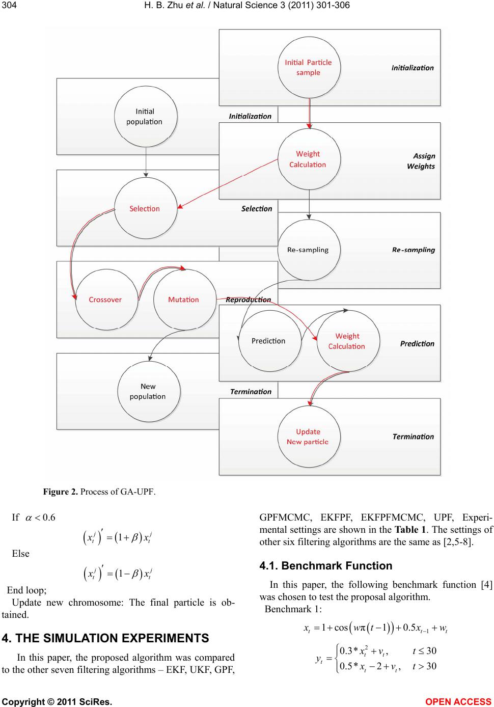
3.3. The GA-UPF Algorithm
In this section, a brief description of UPF is presented
as follow:


11
ijij ij
xtxt vt

 (9)


max min
max
max
t
wwt
ww g

 (10)
The mentioned one-step predefined GA process is
used in the UPF algorithm. The information of UPF al-
gorithm can be found in [3,4]. Where


1, 2,,jDn,


1, 2,,in, n is the size of the
population and Dn is the Dimension of the space sear-
ched; w is the inertia weight, generally updated as
Eq.3 [4], and max
g
is the maximal evolution genera-
tions. 1
c and 2 c are two positive constants. And the
GA-UPF algorithm can be decried as Figure 2.
The detailed process of GA-UPF is as follow:
1) Initial chromosome sample: Draw the new particle
group



, 1,2,,
i
t
x
iNfrom the prior


1tt
pxx
;
2) Assign weights: Every kind of GA has to find an
effective coding scheme. Real matrix encoding is ap-
plied to estimate the parameters for sequential UPF al-
gorithm.
For each loop:
3) Selection: The fitness of each chromosome set as
measuring probability in [5], and using Roulette Wheel
Selection which the most commonly methods to choose
the higher fitness chromosomes, the terminal chromo-
somes is the model of offspring;
4) Crossover: At this stage, arithmetic crossover is
widely used for the chromosome encoded by Real matrix.
In arithmetic crossover, a pair of new individual is gen-
erated by the linear combination of a pair of parent indi-
vidual:




1
1
ii j
tt t
j
ji
tt t
x
xx
x
xx




(11)
Here


0, 1   , ,
ij
tt
x
x is the pair of parent indi-
vidual
 
,
ij
tt
x
x

 is the pair of new individual
5) Mutation:

is a random real;

H. B. Zhu et al. / Natural Science 3 (2011) 301-306 304
Figure 2. Process of GA-UPF.
If 0.6




1
j
j
tt
x
x 

Else


1
j
j
tt
x
x 

End loop;
Update new chromosome: The final particle is ob-
tained.
4. THE SIMULATION EXPERIMENTS
In this paper, the proposed algorithm was compared
to the other seven filtering algorithms – EKF, UKF, GPF,
GPFMCMC, EKFPF, EKFPFMCMC, UPF, Experi-
mental settings are shown in the Table 1. The settings of
other six filtering algorithms are the same as [2,5-8].
4.1. Benchmark Function
In this paper, the following benchmark function [4]
was chosen to test the proposal algorithm.
Benchmark 1:




1
1cos π10.5
ttt
x
wtx w



2
0.3*, 30
0.5*2, 30
tt
t
tt
xv t
yxvt










H. B. Zhu et al. / Natural Science 3 (2011) 301-306 305
Benchmark 2:
 
11
1cos0.04* π*10.5*
ttt
x
txw

 

2sin
0.3* 10
t
kk k
x
yx v
where

3,1
t
w  ,

0,1 4
k
vN e, particle number
N = 200, sample time T = 100, which the results were
the average of 50 times of experiments. 0.5C, R =
1e−4，0.75Q; 1

, 0


, 2k.
4.2. Experimental Results and Remarks
Experimental results are shown in Figures 3, 4 and
Tables 1, 2. All results are the means of 100 runs, as the
results of UPF and GA-UPF are close and far different
with the other algorithms.
As shown in the experimental results, it is clear that,
EKF has the worst results. While the proposed algorithm
has the best results, but has longer running time than
EKF. In theory, the running time of GA-UPF is between
one and two times of UPF, due to the refining step, and it
has been proved by the simulation results.
We extracted a frame from the original video se-
quences per 5 to 10 frames. This is equivalent to in-
crease the speed and uncertainty of target motion, and
Table 1. Results on benchmark 1.
MSE
mean variance
EKF 0.6975 0.1248
UKF 0.3234 0.1297
PF 0.18001 0.1650
PF-EKF 0.1426 0.2147
PF-UKF 0.1239 0.1107
GA-UPF 0.0268 0.0359
Table 2. Results on benchmark 2.
MSE
mean Variance
EKF 0.3375 0.1438
UKF 0.2347 0.1277
PF 0.2301 0.6247
PF-EKF 0.3181 0.1147
PF-UKF 0.2339 0.1347
MPF 0.0968 0.0959
10 12 1416 18 20 22 2426 2830
0
1
2
3
4
5
6
7
8
9
10
Time
Noisy observations
True x
PF
PF-EKF
PF-UKF
GA-UPF
Figure 3. Results on benchmark 1.
10 12 14 16 18202224 26 2830
10
-6
10
-5
10
-4
10
-3
10
-2
10
-1
10
0
Ti me
E rro r
PF
PF-EKF
PF-UKF
GA-UPF
Figure 4. Results on benchmark 2.
then the difficulty level of tracking algorithm is in-
creased. The Experimental result of target tracking is
shown as Figure 5.
In both of the video cameras (Left and Right), the ob-
served images are compared. We can see that tracking
accuracy is in inverse proportion to the distance between
targets and cameras. Tracking errors always occur when
the target is far away from camera, but the performance
shows amazing stability, and the error is within accep-
table limits. The improved algorithm and system can
achieve the desired result.
5. CONCLUSIONS
Basing on the concept of re-sampling, particles with
bigger weights should be re-sampled more time, this
paper has proposed a new type of particle filtering algo-
rithm – GA-UPF. In the GA-UPF, after calculating the

H. B. Zhu et al. / Natural Science 3 (2011) 301-306 306
25 s frame 35 s frame 45 s frame
55 s frame 65 s frame 75 s frame
85 s frame 95 s frame 110 s frame
120 s frame 130 s frame 140 s frame
150 s frame 160 s frame 170 s frame
Left
25 s frame 35 s frame 45 s frame
55 s frame 65 s frame 75 s frame
85 s frame 95 s frame 110 s frame
120 s frame 130 s frame 140 s frame
150 s frame 160 s frame 170 s frame
Right
Figure 5. Sample per 5 frames of tracking video image of binocular vision tracking system.
weight of particles, some particles will join in the refin-
ing process, which means that these particles will move
to the region with higher weights. This process can be
regarded as one-step predefined GA process, so the pro-
posed algorithm is named GA-UPF. Although the GA
process increases the computing load of GA-UPF, but
the refined weights may make the proposed distribution
more closed to the poster distribution. In the following
experiment, the proposed algorithm has better perfor-
mances than other several types of filtering methods.
REFERENCES
[1] Hou, Z.Q. and Han, C.Z. (2005) Based on the back-
ground pixel classification algorithm of reconstructing.
Journal of Software, 16, 1568-1576.
[2] Doucet, A. and Gordon, N. (2001) Sequential Monte
Carlo methods in practice. Springer-Verlag, New York.
[3] Mo, Y.W. and Xiao, D.Y. (2003) Hybrid system monitor-
ing and diagnosing based on particle filter algorithm.
Acta Automation Sinica, 29, 641-648.
[4] Freitas, J.F.G., Niranjan, M., Gee, A.H., et al. (2000)
Sequential Monte Carlo methods to train neural network
models. Neural Computation, 12, 995-993.
doi:10.1162/089976600300015664
[5] Berzuini, C. and Best, N. (1997) Dynamic conditional
independence models and Markov chain Monte Car-
lomethods. Journal of the American Statistical Associa-
tion, 92, 1403-1412. doi:10.2307/2965410
[6] Belviken, E. and Acklam, P.J. (2001) Monte Carlo filters
for non-linear state estimation. Automatica, 37, 177-183.
doi:10.1016/S0005-1098(00)00151-5
[7] Lei, L., Li, Y.-J. and Zhang, K. (2007) A fast algorithm
for searching object centriods in binary images. Infrared
Technology, 29, 548-551.
[8] Higuchi, T. (1997) Monte Carlo filtering using genetics
algorithm operator. Journal of Statistical Computation
and Simulation, 59, 1-23.
doi:10.1080/00949659708811843