Atmospheric and Climate Sciences, 2011, 1, 19-32
doi: 10.4236/acs.2011.12003 Published Online April 2011 (http://www.SciRP.org/journal/acs)
An Examination of the Effects of Aero sol Chemical
Composition and Size on Radiative Properties of
Multi-Component Aerosols
Shaocai Yu*, Yang Zhang
Department of Marine, Earth, and Atmospheric Sciences, North Carolina State University, Raleigh, USA
Received April 11, 2011; revised April 18, 2011; accepted April 19, 2011
Abstract
The sensitivity of aerosol radiative properties (i.e., scattering coefficient, extinction coefficient, single scatter
albedo, and asymmetry factor) and radiation transmission to aerosol composition, size distributions, and rela-
tive humidity (RH) is examined in this paper. Mie calculations and radiation calculations using a tropo-
spheric visible radiation model are performed. The aerosol systems considered include inorganic and organic
ions (e.g., Cl－, Br－, 3 NO

, , Na+,
2
4
SO 
4
NH

, K+, Ca2+, Mg2+, HCOO－, CH3COO －, CH3CH2COO －,
CH3COCOO－, OOCCOO2－, MSA1－), and water-insoluble inorganic and organic compounds e.g., (black
carbon, n-alkanes, SiO2, Al2O3, Fe2O3 and other organic compounds). The partial molar refraction method
and the volume-average method are used to calculate the real and imaginary parts of refractive index of real
aerosols, respectively. The sensitivity simulations show that extinction coefficient increases by 70% when
RH varies from 0 to 80%. Both extinction coefficient and asymmetry factor increase by ~48% when real part
varies from 1.40 to 1.65. Scattering coefficient and single scattering albedo decrease by 18% and 24%, re-
spectively, when the imaginary part varies from –0.005 to –0.1. Scattering and extinction coefficients in-
crease by factors of 118 and 123, respectively, when the geometric mean radius varies from 0.05 to 0.3 m.
Scattering and extinction coefficients and asymmetry factor increase by factors of 389, 334, and 5.4, respec-
tively, when geometric standard deviation varies from 1.2 to 3.0. The sensitivity simulations using a tropo-
spheric visible radiation model show that the radiation transmission is very sensitive to the change in geo-
metric mean radius and standard deviation; other factors are insignificant.
Keywords: Radiative Properties, Sensitivity Study, Aerosol Composition, Aerosol Size Distribution,
Multi-Component Aerosols
1. Introduction
Atmospheric aerosols may influence the Earth’s radia-
tion balance directly by backscattering and absorption
of solar radiation, and indirectly by increasing cloud
condensation nuclei (CCN) concentrations, which in
turn increase cloud droplet concentrations and thus
backscattering of solar radiation [1-3]. The IPCC [4]
concluded that increasing concentrations of the
long-lived greenhouse gases have led to a combined
radiative forcing +2.63 [±0.26] Wm–2, and the total
direct aerosol radiative forcing is estimated to be –0.5
[±0.4] Wm–2, with a medium-low level of scientific
understanding, while the radiative forcing due to the
cloud albedo effect (also referred to as the first indirect
effect), is estimated to be –0.7 [–1.1, +0.4] W

m–2,
with a low level of scientific understanding. Evaluation
of aerosol direct radiative forcing is complicated by the
fact that aerosols are highly and non-uniformly distrib-
uted over the Earth and comprise a variety of chemical
species, and their abundance varies with particle size,
location and time. As indicated by Penner et al. [5], one
of central scientific questions related to the direct radia-
tive influence of aerosols is how the aerosol composi-
tion and size distributions affect the optical depth and
radiative properties of aerosols, including dependence
on relative humidity. Up to today the sensitivity of di-
*Now at AMAD, NERL, U.S. EPA, RTP, NC 27711.

20 S. C. YU ET AL.
rect aerosol forcing to chemical composition, size dis-
tribution and relative humidity on a global scale has
been tested with a “reference box model” [1] and a
GCM model [6-8] Most of these studies except for Ja-
cobson (2001) on direct aerosol forcing only focused on
anthropogenic sulfate aerosols. The objectives of this
paper are 1) to accurately calculate the refractive index
of aerosol particles with the known chemical composi-
tion of atmospheric aerosol; 2) to theoretically evaluate
the sensitivity of aerosol radiative properties and radia-
tion transmission in the visible range to refractive index,
size distributions, and relative humidity (RH) using a
box model that includes Mie and radiative transfer cal-
culation. Since the aerosol particle refractive index is
determined by its chemical composition, the depend-
ence of radiative properties of aerosol particles on the
refractive index can indicate the effects of chemical
composition. Since most of the light scattering and ex-
tinction are caused by particles in the accumulation
mode size range (0.1 - 1.0 m, diameter), and these
particles are neither removed effectively by impaction
nor by diffusion, the accumulation mode particles are
the most important one in terms of aerosol radiative
forcing. In this study the sensitivity of aerosol radiative
properties to size distribution is examined on the basis
of the calculation of the particle radiative properties for
the accumulation mode only.
2. Model Formulation
2.1. Atmospheric Aerosol Composition and Size
Distribution
Atmospheric aerosol particles are composed of complex
mixtures of natural and anthropogenic chemical species
that include 1) water-soluble inorganic and organic
compounds such as sulfate, nitrate, formate and acetate,
2) water-insoluble inorganic and organic compounds
such as black carbon, Al2O3 and n-alkanes, and 3) water
itself. Soluble individual anion and cation concentrations
of atmospheric aerosol are typically measured by Ion
Chromatography (IC), and elements such as Al and Pb
are determined by partially induced X ray emission
(PIXE). On the other hand, the concentrations of insolu-
ble high molecular weight organic compounds in aero-
sols are measured by gas-chromatography-masss pec-
trometer (GS/MS) method [9]. The IC and PIXE meth-
ods provide no information on the concentrations of spe-
cific salts or classes of inorganic and organic salts. The
GC/MS method can quantify the concentrations of indi-
vidual organic compounds in atmospheric particles.
However, only about 10% of the total organic mass can
be typically identified by the GC/MS method [9]. In gen-
eral, the water-soluble materials within atmospheric
aerosol particles are expected to be a mixture of different
chemicals and the water soluble parts of aerosol particles
are considered to be a mixture of electrolytes together
with any other water-soluble material. There are possible
interactions between those ions that do not commonly
exist between chemical components, especially at high
RH conditions [10]. For example, in a mixture of KNO3
and NaCl, there is a possible interaction between K+ and
Na+. It is therefore reasonable to consider water-soluble
parts of aerosol particles as a mixed solute, and aerosol
particles at a dry state composed of mixed solute and
insoluble substances. Since the composition of the aero-
sol particles depends on the sources and subsequent
transformation while airborne, it is possible to separate
aerosols into urban, rural continental and marine aerosols
in a first approximation [11]. Table 1 provides the esti-
mates of refractive index of chemical components for the
three atmospheric aerosol types. The concentrations of
inorganic compounds (Cl－, Br－, 3, NO2
4
SO

, Na+,
4
NH

, K+, Ca2+, Mg2+, SiO2, Al2O3, and Fe2O3), total
concentrations of organics, and total mass concentrations
of aerosol particles for three aerosol types were taken
from the estimates of Pueschel [11]. For organics, over
80 individual organic compounds found in aerosol parti-
cles were identified and quantified previously [9]. In this
study, the concentrations of soluble organic compounds
(HCOO－, CH3COO－, CH3CH2COO－, CH3COCOO－,
2
CCOOOO

, Methane sulfonic acid (MSA)) were taken
from the estimates of Yu [2]. Chylek et al. [12] showed
that the average black carbon (BC) atmospheric concen-
tration in the continental air was 0.23 ± 0.04 g/m3
compared with 0.03 ± 0.01 g/m3 for the maritime air in
the measurements over the southern Nova Scotia.
Huntzicker et al. [13] indicated that the average BC con-
centration for 26 cities in the United State was 3.8 g/m3.
In this study, the BC concentrations used for urban, con-
tinental, and marine aerosols are 3.8, 0.23 and 0.06
g/m3, respectively. The other organic compound con-
centrations listed in Table 1 were taken from the esti-
mates of Roggie et al. [9]. Table 2 lists the physical
chemical and optical properties of various pure salts in
atmospheric particles. For the aerosol model computation,
a lognormal distribution function is suitable to charac-
terize the size distribution of atmospheric aerosols [11].
Particles in the accumulation mode (0.1 - 1.0 m, aero-
dynamic diameter) are the most important one in terms
of aerosol radiative forcing. Table 3 lists the typical size
distributions for three types of aerosol for the accumula-
tion mode at a dry state compiled from literatures. As
shown, the total number concentration, the geometric
mean diameter (Dg), and the geometric standard devia-
tion (g) for the accumulation mode are in the ranges of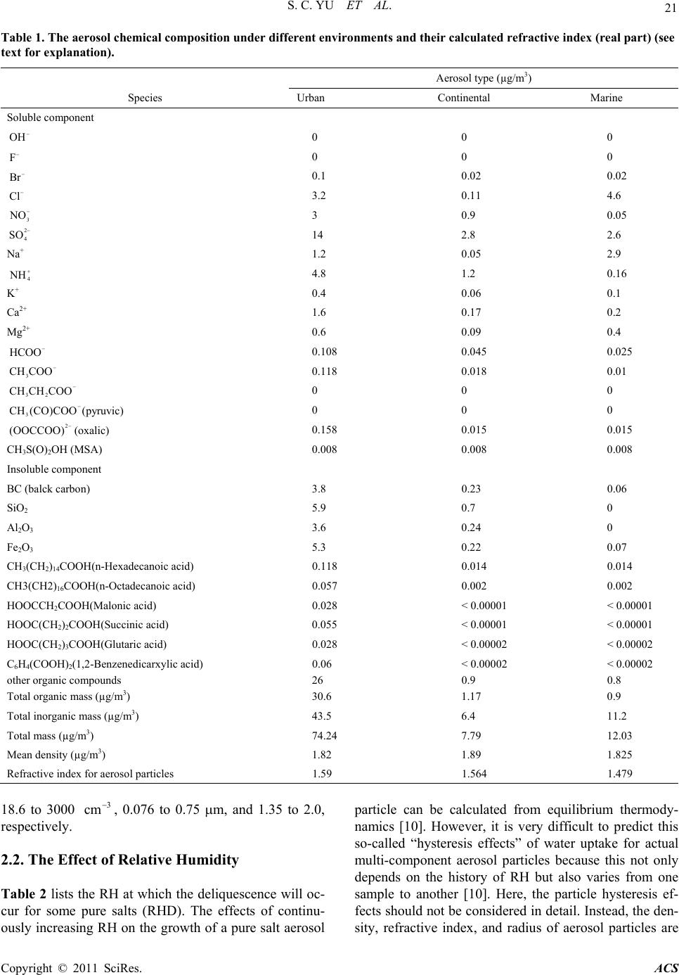

S. C. YU ET AL.
21
Table 1. The aerosol chemical composition under different environments and their calculated refractive index (real part) (see
text for explanation).
Aerosol type (µg/m3)
Species Urban Continental Marine
Soluble component
OH 0 0 0
F 0 0 0
Br 0.1 0.02 0.02
Cl 3.2 0.11 4.6
3
NO
2
3 0.9 0.05
4
SO 14 2.8 2.6
Na+ 1.2 0.05 2.9
4
NH 4.8 1.2 0.16
K+ 0.4 0.06 0.1
Ca2+ 1.6 0.17 0.2
Mg2+ 0.6 0.09 0.4
HCOO 0.108 0.045 0.025
3
CH COO 0.118 0.018 0.01
32
CH CHCOO

0 0 0
3
CH (CO)COO (pyruvic)
2
0 0 0
(OOCCOO) (oxalic) 0.158 0.015 0.015
CH3S(O)2OH (MSA) 0.008 0.008 0.008
Insoluble component
BC (balck carbon) 3.8 0.23 0.06
SiO2 5.9 0.7 0
Al2O3 3.6 0.24 0
Fe2O3 5.3 0.22 0.07
CH3(CH2)14COOH(n-Hexadecanoic acid) 0.118 0.014 0.014
CH3(CH2)16COOH(n-Octadecanoic acid) 0.057 0.002 0.002
HOOCCH2COOH(Malonic acid) 0.028 < 0.00001 < 0.00001
HOOC(CH2)2COOH(Succinic acid) 0.055 < 0.00001 < 0.00001
HOOC(CH2)3COOH(Glutaric acid) 0.028 < 0.00002 < 0.00002
C6H4(COOH)2(1,2-Benzenedicarxylic acid) 0.06 < 0.00002 < 0.00002
other organic compounds 26 0.9 0.8
Total organic mass (µg/m3) 30.6 1.17 0.9
Total inorganic mass (µg/m3) 43.5 6.4 11.2
Total mass (µg/m3) 74.24 7.79 12.03
Mean density (µg/m3) 1.82 1.89 1.825
Refractive index for aerosol particles 1.59 1.564 1.479
18.6 to 3000 , 0.076 to 0.75 m, and 1.35 to 2.0,
respectively.
3
cm
2.2. The Effect of Relative Humidity
Table 2 lists the RH at which the deliquescence will oc-
cur for some pure salts (RHD). The effects of continu-
particle can be calculated from equilibrium thermody-
namics [10]. However, it is very difficult to predict this
so-called “hysteresis effects” of water uptake for actual
multi-component aerosol particles because this not only
depends on the history of RH but also varies from one
sample to another [10]. Here, the particle hysteresis ef-
fects should not be considered in detail. Instead, the den-
ously increasing RH on the growth of a pure salt aerosol sity, refractive index, and radius of aerosol particles are

S. C. YU ET AL.
22
ffernt salts in atmospheric aerosol particles. RHD is the
Index RHD(%)Salts Refractive Index
Density RHD
(%)
Table 2. The physical-chemical and optical properties of di
RH of deliquescence (see text for explanations).
e
Salts Refractive Density
3
(g cm)

 3 (g cm)


NH4O 1.Mg(CH)2(H2O)4 CH3CO 174 3COO 1.491 1.454
NH4Br 1.712 2.429 MgBr 3.724
.423
0 (H2O)5 1.456
3
SO4 1.521 0 )2(H2O)6
4 1.473
)2 .433
2O)
.710 4
2O)6 1.460 3
2
3(H2O)2
OO)2
4
2O)2
4
OO 8 6
8
3(H2O)10
5.3 .320
4(H2O)2
3
4 .240
2O)10
O)
H H2)14COOH
32 16COOH 1.acid
2
450
2
MgCO3 NH4HCO3 11.580 1.717 2.958
NH4Cl 1.642 1.527 8MgCO31.730
NH4F 1.009 MgCl2 1.675 2.320
NH4NO 1.725 62 MgCl2(H2O)6 1.495 1.569
(NH )
4 2
NH4HSO
1.769 8Mg(NO3
MgSO4
1.636
1.780 40 1.560 2.660
Ca(CH COO
3
Ca(Br)
1.550 MgSO4(H2O)7 11.680
3.353 MgSO4(H 1.523 2.445
CaCO
3
CaCO3(H
1.658 2 KBr 1.559 2.750 8
1.771 KCO3
2
K2CO
1.531 2.428 4
CaCl
2
CaCl2(H2O)6
1.520 2.150 31.380 2.043 43
1.417 1.710 KHCO
3
KCl
1.482 2.170
Ca(HC 1.510 2.015 1.490 1.984 88
Ca(NO )(H O)
3 22
CaSO
1.465 1.896 KF 1.363 2.480
4
CaSO4(H2O)2
1.505 2.610 KF(H1.352 2.454
1.521 2.320 K2SO 1.494 2.662
NaCH3C1.464 1.528 7KHSO
4
Pb
1.480 2.322 8
NaBr 1.641 3.203 52.010 11.344
Na CO3
2
Na2CO
1.535 2.532 90 BC 2.000 2.250
1.405 1.440 O
3
SiC
1.223
NaHCO31.500 2.159 2.654 3.217
NaCl 1.544 2.165 7SiO2
H2SO
1.487 2
NaF 1.336 2.558 1.405
NaNO 1.587 2.261 74.5 PbCl
2
Fe O3
2.199 5.850
Na SO
2 4
Na2SO4(H
1.484 2.680 82
Al2O3
3.220 5
1.394 2.680 84 1.768 3.965
NaHSO (H
4 2
CH3CHO
1.460 2.476 52 PbO 2.510 8.000
1.332 0.783 H2O 1.333 1.000
CH3(CH )14COO
2
CH (CH )
1.433 0.853 CH(C
3
formic
1.434 0.853
422 0.941 1.371 1.220
HOOCCH COOH 1.619 acetic acid 1.372 1.049
HOOC(CH2)2COOH 1.1.572 pyruvic acid 1.428 1.227
HOOC(CH2)3COOH 1.419 1.424 oxalic acid 1.900
C6H4(COOH)2 1.431 1.462
Other organics 1.550 1.400
ction of RH in whiche
hysteresis effects” are partially taken into account for
onsidered as a unique func th
“
three aerosol types using the experimental data of Hänel
[10]:

1
0
011
ww
wRH
  

  



(1)
RH 



S. C. YU ET AL.
23
Table 3. Scattering and extinction coefficients, ctor and single scattering albedo and their growth factor for
selected aerosol types. Scattering coefficient (sp ction coefficient (ep, km–1), asymmetry factor (g) and single
attering albedo (). The indices 1,2,3 represent the values at RH=30%, 80% and 99%, respectively. Read
asymmetry fa
, km–1), extin
sc 2
s
1
p
s
p


scattering coefficient at RH = 80% to that at RH = 30%.
as ratio of
coefficient ficient factor
Sin
albedo
Accumulation mode
Scattering Extinction coef-Asymmetry gle scattering
Spectrum Aerosol types
n
–3
Dg g
(cm) (m)
2
1

s
p
s
p

3
1
s
p
s
p


2
1ep
ep


3
1ep


ep 2
1
g
g
3
1
g
g
2
1

 3
1


Meszar Urn 1.1.78.221.12.26 1.0614 os [25]ba560 0.1 2 89 20.76 18 1 1.
W 2300 0 1.72 14.991.66 13.8 1.11 1.29 1.04 1.09
Hoppel 2 1.71 14.471.65 13.341.11 1.28 1.04 1.09
Cl 1.
ta 1.
G] 0.
Schutz [33]
1127 1.
hitby [30]
et al [26]
Continental
Continental
.076
0.08
2
3000
Leaitch and
Isaac [31] ontinenta1000 0.24 351.74 16.761.68 15.571.14 1.39 1.03 1.08
Jenning et al
[32]
athman [27
Continen-
l-marine mix-
ture
950 0.2 351.82 21.521.75 19.751.18 1.53 1.04 1.09
Maritime
Polar aerosol
67 266 1.621.92 16.411.9 16.081.12 1.35 1.01 1.02
Jaenicke and 18.6 0.75 2 1.57 5.53 1.55 5.37 1.06 1.1 1.01 1.03
Average 0.24 1.761.77 15.7871 14.591.12 1.32 1.03 1.08

1

0
011
rrwr rw
w
R
mRH
H
mm m

 




(2 

)

1
0
011 iiwi iw
w
RH
mmm mRH




 



(3)
1
0
011
w
RH
rr RH








where the subscript “w” denotes pure water and “0” in-
dicates the dry substance, mr
imaginary parts of refractive index.
(4)
and mi are the real and

is mean linear
mass increase coefficient. Figure 1 shows

as a func-
tion of RH for three aerosol types, which are obtained
from the experimental results in Table 4 of Hänel [10].
As shown, the dependence of

on RH r difference
types of aerosols is rather complicated. RH can affect
radiative properties of aerosol particles through changing
particle size and refractive ind. Figure 2 shows the
changes of densities, refractive indices, and radius for
three type aerosols as a function of RH. As shown, the
RH effect is important at RH > 80% for density and re-
fractive index, but the radius is sensitive to the change in
RH only when RH > 90%.
3. Results and Discussions
fo
ex
.1. Refractive Index Calculation
ne of central questions for prediction of radiative prop-
ly calculate their
refractive indices. As shown in Table 1, the available
3
O
erties of aerosol particles is to accurate
Figure 1. Mean linear mass increase coefficient (

) as a
function of relative humidity for three typesols
(Maritime aerosols over the Atlantic, 13-16 April, 1969;
Urban aerosols at Mainz, January, 1970; Continental aero-
sols on top of the Hohenpeissenberg, 1000m mean sea level
(MSL), summer, 1970) [10].
partial molar refraction R
of aeros
information on the particle compositions is the ion con-
centrations of soluble components and compound con-
centrations of insoluble components. It has been shown
that the partial molar refraction approach is applicable to
calculate refractive indices for ionic solid-aqueous elec-
trolyte mixtures [14]. The
31
(cm mol

) is defined as [15]:
2
2
1
2
nM
Rn





(5)
where n is refractive index, M is molecular weight, and
  is density (3 gcm

). If the molar refractions of com-
ponents are known, the mean refractive index of a

S. C. YU ET AL.
24
Ta ar refraction of aerosol chemicMH [29
Species
refrtion (Ri, cm–3)
ble 4. The partial molal components. ] is Moelwyn-Hughes [29].
artial molar Ri/Mi Reference P
ac
Soluble components
1 H+ 0 0 MH [29]
2
4 .148 [14]
39 0.237
10 K+ 3.
11 Ca2+ 1.
12 M2+ 0.
13
oxalic)
3S(O)2OH (MSA)
2O 3.71
component
2 7.43
]
2 8.4 .082 telson [14]
]
2)14COOH (n-Hexadecanoic acid)
2)16COOH (n-Octadecanoic acid)
CH2COOH (Malonic acid)
C(CH2)2COOH (Succinic acid)
7
OH 4.43 0.261 MH [29]
3 F 2.17 0.114 MH [29]
Br

 11.84 0Stelson
5 Cl8. Stelson [14]
6 3
NO 10.19 0.164 MH [29]
7 2
SO 
4
+ 0.
13.45 0.14 Stelson [14]
8 Na93 0.04 Stelson [14]
9 4
NH 4.89 0.271 Stelson [14]
03 0.078 Stelson [14]
93 0.048 Stelson [14]
g
HCOO
03 0.001 Stelson [14]
 7.27 0.161 This work
14 3 CH COO 12.94 0.219 This work
15 32
CH CHCOO

17.59 0.241
This work
16 3 CH(CO)COO(pyruvic)
2
17.65 0.203
This work
17 (OOCCOO) (14.53 0.165 This work
18 CH16.82 0.175 This work
19 H
insoluble
0.206 Stelson [14]
20 BC 2.11 0.176 This work
21 SiO0.124 Stelson [14]
22 AlO3
2
Fe O
10.62 0.104 Stelson [14
23 23
PbO
22.210.139 Stelson [14]
410 S
25 Pb 9.24 0.045 Stelson [14
26 CH3(CH 78 0.305 This work
27 CH3(CH 87.29 0.307 This work
28 HOOC17.24 0.166 This work
29 HOO24.2 0.205 This work
30 HOOC(CH2)3COOH (Glutaric acid) 28.40.216 This work
31 C6H4(COOH)2 39.99 0.241 This work
32 other organic compound 50 0.24 This work
mediumn b cae calculated as follows [15]:
1
2
12
R



1



(6)
V
nR 
V 
for an aerosol particle:


C
i
i
i
R
M
R
VAV





(7)
R is the partialr refraction oent i in
1
where i
ol
molaf compon
3
cm m

Mi is thear weightnt i ,
1
mol
molecul of compone
in g

, [Ci] is tcentration oent i in he conf compon
3
mg

 , and [AV] iaerosol volus the me in 3 gm

 .
predicted The aerosol volume can be either measured or
by:

Ci
i
AV


where

i is the density of component i in g cm–3. Table 4
(8)

S. C. YU ET AL.
25
Figure 2. Density, refractive index, and radius as a function
of RH for three types of aerosols.
lists the partial molar refractions for ions. Table 2 con-
tains the refractive index and density for possible salts
found in atmospheric aerosol particles. The refractive
index and density for most compounds in aerosol parti-
cles range from 1.332 to 2.654 and from 0.783 to 11.344
, respectively. Volz [16] reported densities of
luble materials from different rainfalls and loca-
be in a range of 1.76 - 1.96. In this
e average value (1.86 as the
nsity for water-soluble particles.
ty (1.40 ) andx (1.55)
organic comin ken from
lated from:
3
gcm


water-so
tions to
study, th
mean de
The densi
for other
3 gcm


3) is used
rts in aerosol p
e inde
were ta
gcm


a
refractiv
Table 2
3
gcm


pounds
the estimates of Sloane [17]. Additionally, the mean
erosol density,
 , can be calcua i
i
i
s
s




.
tions. T
ed bas
th inter
lar re-
ree aeroso
types at the dry state range from 1.803 to 1.890 g/m3.
In this study, the above partial molar refraction approach
is extended to calculate the refractive index of any at-
mospheric particles with the known chemical composi-
able 4 lists the partial molar refraction for other
aerosol components including insoluble inorganic and
organic compounds, which were calculated on the
method of Weast [15]. In this study, an internal mixture
is assumed for atmospheric aerosol components. Tang
[16] showed that bonal and external mixtures ex-
hibited similar light-scattering properties. Table 1 lists
the values of refractive index and mean density for three
l motypical aerosol types calculated by the partia
fractive approach. The mean densities for thl
The real parts of refractive index for urban, continental,
and marine aerosols are 1.575, 1.557 and 1.479, respec-
tively. As reviewed by Horvath [19], only black carbon
(BC, the main constituent of soot) in atmospheric aerosol
particles is highly absorbed. Hematite (a-Fe2O3) is the
only other substance having a light absorption compara-
ble to EC in the near suggest to use full name of “UV”, u.
v., but absorption rapidly decreases in the visible spec-
trum of the light. There are some discrepancies about the
value of the complex refractive index of EC because of
the difficulty of its experimental determination. The val-
ues given in the literature range from 1.2 to 2.0 for the
real part and from –0.1 to –1.0 for the complex part [19].
In this study, the refractive index used for EC is 2.0 -
0.66i. Since the imaginary parts for all ions in Table 1
are zero and the densities of each ion in Table 1 are not
known, it is not easy to calculate the partial mole refrac-
tions of the ions for imaginary parts using the definition
Equation (5). In this study, the imaginary part of muti-
component aerosols is calculated using the volume aver-
age of the imaginary parts of refractive index of the indi-
vidual species, i
m, as follows [17]:
1
ii
ii
ii
ss
mm



 


 

 

where mi is the imaginary part of refractive index of
component i. With the estimates of BC concentration for
three types of aerosols in Table 1, it was found that the
complex refractive indices for urban, continental and
marine aerosols are 1.575 – 0.027i, 1.557 – 0.016i, 1.479
– .0027i, respectively. Hänel [10] found that the real
part of refractive index for urban aerosols in the city of
Mainz, Germany, was 1.57  0.04 by actual measure-
ment. Grams et al. [20] determined that the complex re-

S. C. YU ET AL.
26
ent this study are very
close to these actual measurements. These complex re-
fractive indices for three types of aerosole used in
the calculation hereafter.
d from 1.55 to 1.90 (average
fficients,
on value
the aerosol
diative properties. The scattering and extinction coeffi-
factor de-
rease by 6% with real part increasing from 1.4 to 1.65.
fractive index for urban aerosols in the city of Boulder,
Colorado O, was 1.55 – 0.044i on the basis of light scat-
tering measurems. The results from
s will b
3.2. The Sensitivity to Relative Humidity
A Mie theory computer code developed by Dave [21] is
used in this study to compute aerosol radiative properties.
All aerosol particles are assumed to be spherical in shape
in the calculation. Ta ble 3 shows the values of the parti-
cle light scattering and extinction coefficients calculated
with the above assumption at RHs of 30%, 80% and 99%
for different particle size distributions of several aerosol
types at a wavelength of 580 nm. The wavelength, 580
nm, is chosen based on the recommendation by Horvath
[19] to give the maximum perception of an object under
the daylight conditions. As shown, the growth factors for
an RH range of 30 to 80% RH range from 1.57 to 1.92
average 1.77 0.12) an(
1.77  0.11) for scattering and extinction coe
espectively. This is in agreement with the criterir
of the hydroscopic growth factor (1.7 0.3) (which is
defined as the ratio of the light scattering coefficient by
an aerosol at an RH of 80% to that at 30%) derived from
the direct nephelometer measurement [22]. This value
has been utilized to date as the first estimate in climate
change modeling studies [1]. It is interesting to note that
Hegg et al. [23] obtained substantially larger values of
the hygroscopic growth (see Table 1 of Hegg et al. [23])
for the same size distribution as those in Table 3. Hegg
et al. [23] attributed it to be influenced by the position of
the initial dry aerosol size distribution relative to the ef-
fective light scattering droplet size range. The main dif-
ferences in our calculation results and those of Hegg et al.
[23] lie in different values of the refractive index and
mean linear mass increase coefficient used for aerosol
particles. The consistence of our results in Table 3 with
the range of hygroscopic growth factor (1.5 to 1.8) from
the direct measurements of Charlson et al. [22] indicates
that our calculation for the effects of RH on scattering
coefficient is reasonable. At a high RH such as 99%, the
growth factors are much higher and more variable than
values at lower RHs as shown in Table 4. The growth
factors range from 1.06 to 1.18 (average 1.12 0.04) and
from 1.10 to 1.53 (average 1.32 0.13) for asymmetry
factor in the RH range of 30% to 80% and 30% to 99%,
respectively. The growth factors range from 1.01 to 1.06
(average 1.03 0.02) and from 1.02 to 1.14 (average
1.08 0.04) for the single scattering albedo in the RH
range of 30% to 80% and 30% to 99%, respectively. The
single scattering albedo is not sensitive to RH. At a high
RH such as 99%, the single scatter albedo is close to 1.0.
The single scattering albedo and asymmetry factor are
insensitive to changes in RH. This is in agreement with
those of Pilinis et al. [24]. Both scattering and extinction
coefficients are more sensitive to changes in RH than
single scatter albedo and asymmetry factor.
3.3. The Sensitivity to Refractive Index
In the following sensitivity studies, the parameters used
for three types of aerosols are assumed to be (1) urban
aerosols of Meszaros [25], N=560 cmm, Dg=0.100
m,

g =2.0, m=1.590 – 0.027i, RH = 80%; (2) conti-
nental aerosols of Hoppel et al. [24], N = 3000 cm–3, Dg
= 0.080 m, 
g = 2.0, m = 1.564 – 0.016i, RH = 80%; (3)
marine aerosols of Gathman [27], N = 67 cm–3, Dg=0.266
m,

g = 1.622, m = 1.479 – 0.003i, RH = 80%. Note
that the values of radius, refractive index in the above
assumptions are for a dry state. RH is set to be 80% in
the Mie calculation. Table 5 lists the ranges and aver-
aged values of the change factors for the effects of real
and imaginary parts of refractive index on
ra
cients increase by about 48% and asymmetry
c
But the single scattering albedo is insensitive to the
changes in real part. Figures 3(a) and (b) show extinc-
tion coefficient and single scatter albedo as a function of
real part of refractive index for three types of aerosols at
a wavelength of 580 nm. Table 5 shows that the scatter-
ing coefficient and single scattering albedo decrease by
18% and 24% when imaginary part varies from –0.005 to
0.10, respectively. The extinction coefficient and asym-
metry factor are insensitive to the change in the imagi-
nary part. As expected, extinction coefficient and asym-
metry factor increase slightly as imaginary part in-
creases.
3.4. The Sensitivity to Size Distributions
As shown in Table 5, scattering and extinction coeffi-
cients are very sensitive to changes in geometric mean
radius. The scattering and extinction coefficients increase
by factors of 118 and 123, respectively, whereas the
asymmetry factor only increases by 17% and the single
scattering albedo decreases by 0.8%, when the geometric
mean radius varies from 0.05 to 0.3 m. Figures 4(a)
and (b) show the sensitivity tests for the case of marine
aerosols at different wavelengths. Table 5 lists the
ranges and averaged changes of radiative properties for
three types of aerosols when geometric standard devia-
tion (g) varies from 1.2 to 3.0. The scattering and

S. C. YU ET AL.
27
Figure 3. The radiative properties at 580 nm as a function of real and imaginary parts of refractive index for three types of
aerosols at a dry state.
Table 5. The change factors for radiative properties of aerosols as a function of real part, imaginary part, geometric mean
radius (rg) and geometric standard deviation (g). The values in parenthesis are the average change factors.
Real part from 1.40 to 1.65 Imaginary part from –0.005 to –0.10rg from 0.05 to 0.3 mm g from 1.20 to 3.0
Scattering coefficient 1.34 - 1.65 (1.49) 0.80 - 0.84 (0.82) 51.5 - 248.5 (118.8) 153 - 753 (389)
extinction coefficient 1.32 - 1.65 (1.47) 1.01 - 1.15 (1.07) 59.2 - 249.3 (123.7) 155 - 607 (334)
1.00 - 1.01 (1.01) 0.79 - 0.73 (0.76) 0.87 - 1.00 (0.92) 0.99 - 1.24 (1.1)
Asymmetry factor 0.92 - 0.95 (0.94) 1.03 - 1.01 (1.02) 1.09 - 1.32 (1.17) 3.1 - 8.3 (5.4)
Single scattering albedo
extinction coefficients and asymmetry factor are very
sensitive to the change in geometric standard deviation.
aerosol size distribution when geometric mean radius
varies from 0.1 to 0.4 m at N0 = 560 cm–3
The scatteng and ex
factors of 89.3 and 3
stries fhis change
gease octor by a fact
of rease ong albedo
1d sensitivity
symmetry factor and single scattering albedo to changes
and g = 2.0
metriion
0 .
e light sca of aar-
ependent e, win-
urring betw7 m iius
wavelen, aeroan
have large scattering and extinction coefficients if their
ri
3
tinction coefficients inc
34, respectively, when
rease by
geometric
and when geo
to 3.0 at N = 5
andard deviation varom 1.2 to 3.0. Tof Since th
results in the incrf asymmetry faor ticle is d
5.4 and the incf single scatteriby cies occ
0%. Figures 4(c) an(d) show the of for a light
c standard deviat
60 cm–3 and r= 0.15
varies from 1.2
m, respectively
g
ttering efficiencyn individual p
on the particle sizth peak efficie
een ~0.2 and 0.n particle rad
gth of 580 nmsol particles c
a
in g values for urban aerosols at different wavelengths.
Figure 5(a) and (b) show the changes of the shape of
size distributions grow into this efficient light scattering
size range. Figure 5 indicates that both cases can result

28 S. C. YU ET AL.
Figure 4. The radiative properties at 580 nm as a function of geometric mean radius (for Gathma’s maritime aerosols (a, b),
and geometric standard deviation (for Meszaros’ urban aer osols (c , d)).
(a) (b)
Figure 5. The size distribution of aerosol number concentration as a function of geometric mean radius (a) and standard de-
viation (b).

S. C. YU ET AL.
29
in more particles in the efficient light scattering size
range (with radii of 0.2 to 0.7 m). It is not surprised to
find that the scattering and extinction coefficients are
very sensitive to the changes in geometric mean radius
and geometric standard deviation.
3.5. The Sensitivity of Wavelength Dependence
of Radiative Properties
The wavelength dependence of aerosol radiative properties
is very sensitive to geometric mean radius. When the
geometric mean radius is small, both single scattering
albedo and asymmetry factor decrease with increasing
wavelengths, but when the
comes larger than a value, both single scat
he latter case, the Angstrom law will not be
light scattering effi-
iency of an individual particle is a nonlinear function of
t
wavtive index is wavelength
ependent, the wavelength dependence of aerosol radia-
metric standard deviation is weak. For small geometric
mean radius and small geometric standard deviation,
both asymmetry factor and single scattering albedo in-
crease with decreasing wavelengths, however, for large
values of geometric mean radius and geometric standard
deviation, both asymmetry factor and single scattering
albedo increase with increasing wavelengths, especially
for single scattering albedo, as shown in Figure 4.
3.6. Radiation Transmission
Since human-induced aerosols are likely to greatly in-
fluence future regional climate change instead of global
amine the sensitivity
nsmission changes at
tributions, and RH. In this study, the radiation transmis-
nm is
amined under the following constant conditions: date =
lbedo = 0.15, air pres-
ure = 940 mb, Latitude = 35.63˚, longitude = 82.33˚, UT
radiative transfer model for different aerosol types assuming
atit .90, zenith ang
geometric mean radius be-
tering albedo
climate change, it is of interest to ex
of the aerosol-induced radiation tra
and asymmetry factor increase with increasing wave-
engths. For t
a local or regional scale to aerosol composition, size dis-
l
applicable. The values of geometric mean radii at the
crossing point are different for asymmetry factor and
single scattering albedo as shown in Figures 4(a) and (b),
and are also determined by the geometric standard devia-
tion as analyzed below. Since the
c
particle size and depends on the particle size and ligh
elength tested, and the refrac
d
tive properties will strongly rely on the size distribution
and refractive index. For the wavelength dependence of
refractive index, available data were closely matched by
setting n() = n( = 0.598 m) – 0.03( – 0.598), where
is the wavelength in m. As shown, the wavelength
dependence of refractive index is weak. As shown in
Figure 4, the wavelength dependence of asymmetry fac-
tor and single scattering albedo strongly relies on the
geometric mean radius and geometric standard deviation.
But the wavelength dependence of scattering and extinct-
tion coefficients on the geometric mean radius and geo-
sion is calculated for the assumed aerosol layer with a
depth of 2 kilometers using the Madronich’s Tropo-
spheric Ultraviolet-Visible Radiation Transfer Model
(TUVRTM) [28]. The optical depth

2
1
d
z
e
z
zz  is
calculated by assuming a constant extinction coefficient
within the aerosol layer. The sensitivity of aero-
sol-induced radiation transmission changes at 580
Table 6. The radiation transmission at 580 nm calculated by a
an aerosol layer of 2 km. The date is 7/1/1995, O3 = 278 DU, l
13.31˚.
Accumulation mode
ex
7/01/1995, O3 = 278 DU, ground a
s
= 17.90, solar zenith angle = 13.31, the aerosol layer = 2
km. Three aerosol radiative properties (optical depth,
asymmetry factor, and single scattering albedo) are
needed in the TUVRTM model to calculate the aero-
sol-induced radiation transmission changes. In this sec-
tion, the sensitivity of the aerosol-induced radiation
transmission change to RH, refractive index, and size
distribution is studied based on previous calculation re-
ude = 35.63˚, longitude = –82.33˚, UT = 17le =
Transmission at 580 nm
Spectrum Aerosol types n (cm–3) Dg (μm) σg T1 (RH=30)T2 (RH=80) T1 (RH=99) T2/T1 T
3/T1
Meszaros [23] Urban 560 0.1
Whitby [28] Continental 2300 0.076
Hoppel et al [24] Continental 3000 0.08
Leaitch and Isaac [29] Continental 1000 0.24
Jenning et al [30] Continental-
marine mixture 950 0.2
Gathman [25] Maritime 67 0.266
Jaenicke and Schutz [31] Polar aerosol 18.6 0.75
Background without aerosol
layer 0 0
2
2
2
1.3
1.3
1.6
2
0
0.908 0.908 0.906 1 1
0.906 0.906 0.890 1 0.98
0.904 0.895 0.840 0.99 0.93
5 0.897 0.895 0.844 1 0.94
50.904 0.903 0.876 1 0.97
20.911 0.911 0.911 1 1
0.910 0.911 0.911 1 1
0.911 0.911 0.911

S. C. YU ET AL.
30
nm
for three types of aerosols.* The average is calculated only for ban and continental aerosols.
Table 7. The change factors for radiation transmission at 580 as a function of relative humidity and radiative properties
ur
Aerosol type
Parameter Urban Continental Marine average*
Relative humidity from 0 to 95% 0.999 0.993 1 0.996
Real part fro 1.40 to 1.65 0.992 0.995
Imaginary part from –0.005 to –0.100.9
Numbeom 0.958
.30 μm 0.467 2 0.99
.0 0.934 1 0.997
m0.998
0.979
1
67 0.998 0.973
r concentrations fr 50 to 4000 cm-3 0.94 0.977 77 0.9
rg from 0.05 to 0
σ from 1.2 to 3
0.02
0.83
0.244
0.883
g
Figure 6. The radiation transmission at 580 nm across an aerosol layer with a 2-km in depth as a function of RH, real and
imaginary parts, number conce ntration, and size distribution for three types of aerosols.

S. C. YU ET AL.
31
sults of aerosol radiative properties for the three types of
aerosols. Table 6 lists the radiation transmissions at 580
nm for different aerosol types at RHs of 30%, 80% and
99%. Figure 6 shows the sensitivity of radiation trans-
mission to RH, refraction index, number concentrations
and size distributions for the three types of aerosols. Ta-
ble 7 lists the change factors for radiation transmission
for three types of aerosols. Note that the radiation trans-
mission at 580 nm is 0.911 without the aerosol layer un-
der the assumed atmospheric conditions. It is interesting
to note that the radiation transmission is not sensitive to
the changes in the above parameters if the total aerosol
number concentration is small as it for maritime aerosols
of Gathman [27] (total number concentration is only 67
cm–3 as indicated in Table 7). In this case, the radiation
transmission only decreases by 0.4% and 0.5% when RH
varies from 0% to 95% and the real part varies from 1.40
to 1.65, respectively. The radiation transmission is sensi-
tive to the change in imaginary part and number concen-
trations with the decrease of visible radiation transmis-
sion by 2.7% and 4.2% when the imaginary part varies
from –0.005 to –0.1 and number concentration from 50
to 4000 cm–3, respectively. The radiation transmission is
very sensitive to the changes in geometric mean radius
and geometric standard deviation. The radiation trans-
mission decreases by 76% when geometric mean radius
varies from 0.05 to 0.3 m and decreases by 12% when
geometric standard deviation varies from 1.2 to 3.0. This
is in agreement with the strong dependence of scattering
and extinction coefficients on geometric mean radius and
geometric standard deviation. It should be emphasized
that the radiation transmission also strongly depends on
the solar zenith angle, latitude and longitude, and ozone
concentrations.
4. Conclusions
In this work, the partial molar refraction method is used
to accurately calculate the real part of refractive index of
aerosol particles with actual measured chemical compo-
sitions including soluble inorganic and organic ions and
dius and geometric standard deviation of a particle size
distribution. The radiation transmission decreases by
76% and 12% when geometric mean radius varies from
0.05 to 0.3 m and geometric standard deviation varies
from 1.2 to 3.0, respectively. Other sensitivities for the
radiation transmissions are insignificant. The comparison
between theoretical calculation and actual measurement
will be necessary in the future work.
5. References
[1] R. J. Charlson, S.E. Schwartz, J. M. Hales, R. D. Cess, J.
A. Coakley, J. E. Hansen and D. J. Hofmann, “Climate
Forcing by Anthropogenic Aerosols,” Science, Vol. 225,
1992, pp. 423-430.
doi:10.1126/science.255.5043.423
insoluble inorganic and organic substances. It is found
hat the complex refractive indices for urban, continental t
and marine aerosols are 1.575 – 0.027i, 1.557 – 0.016i
and 1.479 – 0.003i, respectively. The scattering and ex-
tinction coefficients are sensitive to changes in RH,
while both single scattering albedo and asymmetry factor
are insensitive to change in RH. The extinction coeffi-
cient and asymmetry factor are sensitive to changes in
real part of refractive index. The scattering coefficient
and single scattering albedo are sensitive to the imagi-
nary part changes. The aerosol radiative properties are
very sensitive to the change in both geometric mean ra-
[2] S. C. Yu, “The Role of Organic Acids (Formic, Acetic,
Pyruvic and Oxalic) in the Formation of Cloud Conden-
sation Nuclei (CCN): A Review,” Atmospheric Research,
Vol. 53, 2000, pp. 185-217.
doi:10.1016/S0169-8095(00)00037-5
[3] S. C. Yu, V. K. Saxena and Z. Zhao, “A Comparison of
Signals of Regional Aerosol-Induced Forcing in Eastern
China and the Southeastern United States,” Geophysical
Research Letters, Vol. 28, 2001, pp. 713-716.
doi:10.1029/2000GL011834
[4] Intergovernmental Panel on Climate Change (IPCC),
“Climate Change 2007: The Physical Science Basis,”
Contribution of Working Group I to the Fourth Assess-
ment Report of the Intergovernmental Panel on Climate
Change, Cambridge University Press, New York, 2007.
[5] J. E. Penner, R. J. Charlson, J. M. Hales, N. S. Laulainen,
R. Leifer, T. Novakov, J. Ogren, L. F. Radke, S. E.
Schwartz and L. Travis, “Quantifying and Minimizing
Uncertainty of Climate Forcing by Anthropogenic Aero-
sols,” Bulletin of the American Meteorological Society,
Vol. 75, 1994, pp. 375-400.
doi:10.1175/1520-0477(1994)075<0375:QAMUOC>2.0.
CO;2
[6] O. Boucher and T. L. Anderson, “General Circulation
Model Assessment of The Sensitivity of Direct Climate
Forcing by Anthropogenic Sulfate Aerosols to Aerosol
Size and Chemistry,” Journal of Geophysical Research,
Vol. 100, 1995, pp. 26117-26134.
doi:10.1029/95JD02531
[7] M. Z. Jacobson, “Global Direct Radiative Forcing Due to
Multicomponent Anthropogenic and Natural Aerosols,”
Journal of Geophysical Research, Vol. 106, 2001, pp.
1551-1568. doi:10.1029/2000JD900514
[8] D. Koch, S. Bauer, A. Del Genio, G. Faluvegi, J. R.
McConnell, S. Menon, R. L. Miller, D. Rind, R. Ruedy,
G. A. Schmidt and D. Shindell, “Coupled Aero-
sol-Chemistry-Climate Twentieth Century Transient
Model Investigation: Trends in Short-Lived Species and
Climate Responses,” Journal of Climate, 2011.
[9] W. F. Rogge, M. A. Mazurek, L. M. Hildemann, G. R.
Cass and B. R. T. Simoneit, “Quantification of Urban

32 S. C. YU ET AL.
Organic Aerosols at a Molecular Level: Identification,
Abundance and Seasonal Variation,” Atmospheric Envi-
ronment, Vol. 27, 1993, pp. 1309-1330.
[10] G. Hänel, “The Properties of Atmospheric Aerosol Parti-
cles as Functions of Relative Humidity at Thermody-
namic Equilibrium with the Surrounding Air,” Advances
in Geophysics, Vol. 19, 1976, pp. 73-188.
doi:10.1016/S0065-2687(08)60142-9
[11] R. F. Pueschel, “Atmospheric Aerosols,” In: Singh H.
B.,Van Nostrand Reinhold, Eds., Composition, Chemistry
and Climate of the Atmsopher, 1995, pp. 120-175.
[12] P. Chylek and J. Wong, “Effect of absorbing aerosols on
global radiation budget, Geophysical Research Letters,
Vol. 22, No. 8, 1995, pp. 929-931.
doi:10.1029/95GL00800
[13] J. J. Huntzicker, R. L. Johnson, J. J. Shah and R. A. Cary,
“Analysis of Organic and Elemental Carbon in Ambient
Aerosols by a Thermal-Optical Method,” In: Particulate
a Particle Trap Impac-
mpler, Environmental Science & Tech-
nology, Vol. 35, No. 24, 1982, pp. 4857-4867.
Carbon: Atmospheric Life Using
tor/Denuder Sa
[14] A. W. Stelson, “Urban Aerosol Refractive Index Predic-
tion by Partial Molar Refraction Approach,” Environ-
mental Science & Technology, Vol. 24, 1990, pp.
1676-1679. doi:10.1021/es00081a008
[15] R. C. Weast, CRC Handbook of Chemical and Physics,
Cleveland, OH, 1988.
[16] F. Volz, “Infrared Absorption by Atmsopheric Aerosol
Substances,” Journal of Geophysical Research, Vol. 77,
1972, pp. 1017-1031. doi:10.1029/JC077i006p01017
[17] C. S. Sloane, “Optical properties of aerosols of mixed
composition,” Atmospheric Environment, Vol. 18, 1984,
pp. 871-878. doi:10.1016/0004-6981(84)90273-7
[18] I. N. Tang, W. T. Wong and H. R. Munkelwiz, “The
Relative Importance of Atmospheric Sulfates and Nitrates
in Visibility Reduction,” Atmospheric Environment, Vol.
15, 1981, pp. 2463-2471.
doi:10.1016/0004-6981(81)90062-7
[19] H. Horvath, “Atmospheric Light Absorption - a Review,”
Atmospheric Environment, Vol. 27, 1993, pp. 293-317.
[20] G. W. Grams, I. H. Blifford, D. A. Gillette and P. B. Rus-
sell, “Complex Index of Refraction of Airborne Soil Par-
ticles,” Journal of Applied Meteorology, Vol. 13, 1974,
pp. 459-471.
doi:10.1175/1520-0450(1974)013<0459:CIOROA>2.0.C
O;2
[21] J. V. Dave, “Subroutines for Comp
of Electomagnetic Radiation Scatter
uting the Parameters
ed by a Sphere,”
0302
IBM
Journal of Research and Development, Vol. 13, 1969, pp.
302-312. doi:10.1147/rd.133.
on, “Observa-
tical Study
idity on Light Scattering by
[22] R. J. Charlson, D. S. Covert and T. V. Lars
tions of the effect of humidity on light scattering by
aerosols,” In: Ruhnke T. H. and Deepak A., Eds., Hygro-
scopic Aerosols, pp. 35-44, Hampton, VA, 1984.
[23] D. Hegg, T. Larson and P. F. Yuen, “A Theore
of the Effect of Relative Hum
Tropospheric Aerosols,” Journal of Geophysical Re-
search, Vol. 98, 1993, pp. 18435-18439.
doi:10.1029/93JD01928
[24] C. Pilinis, S. N. Pandis and J. H. Seifeld, “Sensitivity of
Direct Climate Forcing by Atmospheric Aerosols to
Aerosol Size and Composition,” Journal of Geophysical
Research, Vol. 100, 1995, pp. 18739-18754.
doi:10.1029/95JD02119
[25] A. Meszaros, “On the Concentration and Size Distribu-
tion of Atmospheric Sulfate Particles under Rural Condi-
tions,” Atmospheric Environm
2425-2428.
ent, Vol. 12, 1978, pp.
doi:10.1016/0004-6981(78)90286-X
W. A. [26] Hoppel, R. Larson and M. A. Vietti, “Aerosol Size
Distributions at a Site on the East Coast of the United
States,” Atmospheric Environment, Vol. 18, 1984, pp.
1613-1621. doi:10.1016/0004-6981(84)90383-4
[27] S. C. Gathman, “Optical Properties of the Maritime
Aerosols as Predicted by the Navy A
tical Engineering, Vol. 22
erosol Model,” Op-
, 1983, pp. 56-62.
ag, Amsterdam,
[28] S. Madronich, “Tropospheric Photochemistry and Its
Response to UV Changes,” In: M. L. Chanin, Ed., The
role of the stratosphere in global change, NATO-ASI Se-
ries, Vol. 18, pp. 437-461, Springer-Verl
1993.
[29] E. A. Moelwyn-Hughes, Physical Chemistry, 2nd rev. ed.,
Pergamon Press, New York, 1961.
[30] K. T. Whitby, “The Physical Characteristics of Sulfur
Aerosols,” Atmospheric Environment, Vol. 12, 1978, pp.
135-159. doi:10.1016/0004-6981(78)90196-8
[31] W. R. Leaitch and G. A. Isaac, “Tropospheric Aerosol
Size Distributions from 1982 to 1988 over Eastern North
America,” Atmospheric Environment, Vol. 25, 1991, pp.
601-619.
[32] S. G. Jennings, C. D. O’Dowd, T. C. O’Connor and F. M.
McGovern, “Physical Characteristics of Ambient Aerosol
at Mace Head,” Atmospheric Environment, Vol. 25A,
1991, pp. 557-562.
[33] R. Jaenicke and L. Schiitz, “Arctic Aerosol in Surface
Air,” ldoyaras 86, 1982235-241.