Journal of Geographic Information System, 2011, 3, 128-139
doi:10.4236/jgis.2011.32009 Published Online April 2011 (http://www.SciRP.org/journal/jgis)
Dynamic-Distributed Load Balancing for
Highly-Performance and Responsiveness
Distributed-GIS (D-GIS)
Aissatou Diasse1,2, Foroski Kone1,2
1Faculty of Information Engineering, China University of Geosciences, Wuhan, China
2GIS Software and Application Research Center of Ministry of Education, Wuhan, China
Received January 10, 2011; revised February 2, 2011; accepted Febr uary 15, 2011
Abstract
In recent years, several results have been introduced to enhance distributed GIS performance. While much
more efforts have focused on tile map and simple symbologies on dynamic map, load balancing GIS servers
have not been addressed by the GIS community so far. This paper, therefore, proposed dynamic distributed
load balancing for D-GIS in order to quickly render information to client interface by involving a set of GIS
servers which process clients’ requests depending of an algorithm. In the model, several concepts were in-
troduced and defined: Virtual Server within physical machine which constitutes a setup environment for a
single GIS server, Load Hash Table which contains information about virtual server’s capacity, real-time
load and other mandatory elements, Request Split Table which splits requests depending of the input area’s
Quantity of Information and stores request tasks composition for later reconstitution. At last we have Dis-
tributed Failover Callback Function Table level one (respectively level two) which determines whether or
not the request had been successfully processed by the chosen virtual server (respectively physical machine).
This table allows sending back the same request to another virtual server (respectively physical node). Two
load handlers (primary and secondary) are defined in case of failure. Our Model achieves efficient load bal-
ancing by: providing efficient node selection; optimizing request routing; managing node failover; involving
client’s request partitioning and introducing method type decomposition. A simulation of the algorithm
shows a low response time when performing GIS operations.
Keywords: Load Balancing, Distributed-GIS, Performance, Responsiveness
1. Introduction
1.1. History
A centralized GIS, which provides an environment for
desktop or standalone application is traditionally use.
Now with the growth of internet techniques, D-GIS
which are based-on distributed system are being used
much more in place of traditional GIS. These systems
used tens or hundreds of computers connected by high
speed networks and have many advantages over stand-
alone computers [1,6,7]. They provide resource sharing
as one of their major advantages, which bring better per-
formance and reliability than any other traditional system
in the same conditions [2]. Like distributed system,
D-GIS are composed of autonomous hosts that are con-
nected through a computer network [3]. They aim shar-
ing of data and computation resources and collaboration
on large scale applications [4]. Thus, the architecture of
D-GIS is different from of traditional GIS because the
system is built on the open and distributed internet envi-
ronment [5]. D-GIS has two advantages. Firstly, they are
designed with tools and features that are common to
webpage and secondly they allow the dissemination of
geographic data to multitude of clients and provide, ac-
cess and perform GIS functions in the web.
1.2. Problems
Even with these advantages, recent use of this system

A. DIASSE ET AL.129
shows that there exist shortcomings that D-GIS commu-
nities are faced. One of the critical problems faced is that
of serving resources for multitudes of clients which has
as consequence the decrease of performance and respon-
siveness of the applications. These are due among other
to (1) islands of technology used, (2) large among of data
transfer over the internet, (3) numerous remote calls to a
single GIS server and numerous heterogeneous devices.
However, since productivity and efficiency are the busi-
ness forces of organizations, GIS providers must seek for
ways to break down the cause of low performance.
Several methods have been used to enhance D-GIS
performance. One of such methods is the use of new data
organization known as Tile Map, to reduce the data dis-
playing and retrieving time. Nevertheless, very few
studies had been focus on the load balancing of D-GIS
servers which is one of the most successful methods to
enhance applications performance in distributed systems
computing. For those GIS systems that integrate load
balancing into their applications, static load balancing is
used which is inappropriate for D-GIS where tasks re-
quirements’ capacity vary frequently.
1.3. Contributions
In this paper we investigated, studied and designed dy-
namic load balancing algorithm for distributed GIS. We
discussed and illustrated the use of virtual servers and
double load balancer handlers. The system failover is
managed by the introduction of two tables at two system
levels to overcome virtual servers and physical machines
failover. Moreover a request split style and a method-
decomposition are proposed to further enhance the per-
formance of GIS applications. By taking as prototype a
dynamic load balancing algorithm in peer to peer system,
we modify, adjust and add some innovative parameters
and tables on the algorithm to present a dynamic load
balancing for distributed GIS systems.
1.4. Method
Firstly we defined and described the proposed model for
balancing users’ requests into a GIS servers cluster in
section 2. Secondly, we went deeply into the model de-
scription with the different parameters, components, as-
sumptions, architecture and algorithms. Finally we pro-
posed a prototype implementation model of our distrib-
uted GIS system with the different distributed tiers. The
simulation showed that the model fairly optimized the
performance and responsiveness of the implemented
applications based on our D-GIS designed and provided
high availability in a scalable manner to meet future
needs.
2. Overview
For proposing an efficient load balancing model for dis-
tributed GIS systems, we investigated some issues for a
better responsiveness of implemented application.
 How can we balance the user’s request between the
GIS servers in the cluster efficiently?
 How can we handle client information that must be
kept across the multiple requests?
 Is it the load balancing of the users’ processes
composed of several GIS tasks?
 How do we process the load balance when a re-
quest is composing of different GIS tasks?
 Where do we run a new job in the cluster when
there is equal load on the different nodes?
 Are the costs to process a request the same regard-
less of which nodes are involved?
 Is the transfer of users’ incoming request costless?
Can it be negligible?
To implement the model for a satisfaction of the above
statements, we impose to the distributed layers within the
system to be balanced using an appropriate algorithm.
Each layer is composed of several servers called cluster
servers. The load balancer allows client’s access to the
cluster servers using a common domain name with a sin-
gle virtual IP address. The load-balancing algorithm in-
tercepts the incoming HTTP traffic and directs it to one
of the servers in the cluster.
After deep study and considerations, we thought that
the algorithms must be implemented in two different
levels to provide highly available performance and re-
sponsiveness. The two cluster servers are the GIS servers
cluster and the GIS services cluster. The first cluster
contains the GIS services which balance users’ requests
using the Network Load Balancing. This method is not
covered in this paper. The second cluster contains the
GIS servers which use Dynamic Distributed Load Bal-
ancing (DDLB) algorithm. The paper is about the load
balancing into GIS servers cluster.
3. Dynamic-Distributed Load Balancing
Model on GIS Servers Cluster
3.1. Model Definition
In this section, we define the model proposed to balance
the GIS servers cluster. A dynamic algorithm is used to
balance user’s requests. The algorithm uses the concept
of virtual servers [11-16] to host processes. The basic
idea of the model is to divide the machines into several
virtual servers, store their information into a well known
table called Load Hash Table (LHT) which is frequently
updated to restore the real time nodes load, server

A. DIASSE ET AL. 130
failover likelihood and so on. When client requests a
process provided by the GIS server, the LHT is used by
the algorithm to search the appropriate virtual server and
then send the client request to that specific server. If re-
quest is a getMap() or getInfo-OnInputArea() functions,
input area is split depending of the area quantity of in-
formation. The proposed algorithm uses the utilization of
the node instead of its load because virtual servers might
in real life have heterogeneous capacity. However their
capacity is used to balance the first incoming client re-
quest.
3.2. Model Description
For the GIS server cluster we proposed a dynamic load
balancing algorithm which used a LHT as match up sys-
tem between the nodes of the cluster and their utilizing
load at any given time. The algorithm balances the cli-
ents’ requests to nodes in the cluster, which yields a
load-balanced system when the LHT maps nodes effi-
ciently into the corresponding weight-load. The LHT is a
concept we introduce in our distributed GIS that follow
the hash table paradigm (HT). The HT or hash map is a
data structure that uses a hash function to efficiently map
certain identifiers or keys to associated values [17].
Whenever a specific virtual server is chosen it is stored,
together with the client request in a table call distributed
failover callback function table (DFCFT). This table al-
lows the system to manage failover. The DFCFT con-
tains the request status field which allows the parent
node to be aware of the successful process and send the
request to another node. However before processing cli-
ent request the split request function is used to split client
request into simple tasks and store the different tasks into
a Split Request Table (SRT) in order to reconstitute the
original request and render appropriate response. The
dynamic distributed load balancing algorithm is charac-
terized by a set of criteria describe in the follow points.
 Scalability: The node can be increased and de-
crease as wanted. Therefore even with ten, thou-
sands or millions of virtual nodes the system will
work correctly.
 Semi-Distributed: Each physical node has a copy
of the DCFT in its memory and a general real time
update must be done to update the tables in each
node.
 Centralization: The nodes are collectively taken as
slave node with a central coordination call master
node. System store global information in the load
balancer, so any of the slave nodes cannot be a
master node.
 Fault Tolerance: The system is reliable; in fact the
LHT, even with failover, continuously maps spe-
cific nodes with a Upper Loaded: Upper Loaded =
C + & such & > 0
 Availability: Even when servers within the cluster
fail, the remaining servers are performing normally
and can take over the failing server’s request using
either physical node level or cluster node level.
 Affinity: The system can manage a user's requests,
either to a specific server or any server, depending
on whether session information is maintained on
the server or at an underlying database level.
 Adaptive: the algorithm is adapted to each incom-
ing request due to the division of input area based
on its quantity of Information.
 Bi-Load Balancers: The system is composed of
two load balancers. For high-availability we pro-
posed a primary load balancing and a secondary in
case the load balancer fails.
3.3. Model Composition
3.3.1. Virtual Server (VS)
By using a known dynamic load balancing with setup
servers on physical machines, client request is balanced
within the different servers. These servers are character-
ized by their capacity which is different from one another
and their load is determined by performing client tasks.
Although the load balancing used on these servers may
be efficient to balance the users’ requests, the load pro-
vided by each physical node may not be efficient for a
highly performance server utilization. Hence, load algo-
rithm methods which use physical machine do not evenly
partition the load to nodes. Therefore some machines get
a big users’ request depending on their capacity while
other get small requests which flout the load balancing
characteristics.
To overcome this shortage we introduced the concept
of virtual servers in our farmer GIS servers for each
computer. A virtual server is a completely isolated con-
tainer capable of processing operation system and appli-
cations [18], behave like a physical machine and contains
its own CPU, RAM, hard disk and interface card. It
represents a node in the LHT in which routing, storage or
retrieval of data items happen rather than at the physical
node. Heterogeneity of node capacity is the main reason
of using virtual servers per node than in the equal-ca-
pacity case, thus increasing the scalability of the system.
Each virtual server node in the cluster is seeing itself as a
physical device. A physical computer hosts one or more
virtual servers depending of it capacity, it potential of
failover, and load balancing is achieved by moving load
from heavily to lightly VS nodes. When dividing physi-
cal machines into virtual servers, we must choose care-
fully the number of virtual servers to create since a huge

A. DIASSE ET AL. 131
number of virtual servers within a physical node may
reduce the performance of the application system. One of
the main repercussions of using virtual servers is the
considerable reduction in the number of hardware com-
puters used and the optimization of waste for capacity
un-used on a single computer. Nevertheless the draw-
back of the utilization of these virtual servers increase
the bandwidth and storage requirement [14] but this con-
sideration is not great compared to the advantages.
(RTJP) & Real-Time-Successful-Process (RTSP). The
RTWL is the real time load of a particular virtual server
node. This is given by providing a web services script
that calculates the virtual server process time at any min-
ute and writing down into the loaded hash table. The
RTJP is the real time set of jobs being processed by any
particular node. The RTSP is the real time successful
process provide by any node within the cluster. Within
the LHT, we initialize the node with static values such as
CI, the capacity of the virtual server I (VSI); UL, the Up-
per Loaded value that when a node receive that quantity
of work it considered itself over-loaded; LL, the Lower
Loaded value that when a node receive that quantity of
work it considered itself under-load. The LHT also pro-
vides the VSI Physical Node Membership (PNM) and
Failover Likelihood (FL) of each virtual server to deter-
mine the probability of its failover which depends of the
node’s previous failover (Table 1).
3.3.2. Load Balancer
The system provides two load balancers, a primary load
balancer which handles load balancing between the sev-
eral GIS servers within the cluster and a secondary load
balancer in case the primary load balancer failed. It lev-
erages the servers’ nodes to enhance responsiveness.
Each VS node is configured to use the load balancers and
will periodically send load and other information to the
activated load balancer which will keep track of the load
and availability of each VS node to which it is commu-
nicating (see LHT section below). Physical machines are
also configured to use the load balancers and will allow
the load balancer to get information about client request
status whenever it is able to successfully perform the
incoming request from the load balancer. The latter will
keep track of the successful processing of each physical
machine to which it is communicating in order to resend
the same tasks to another physical node in case of
failover. Since two load balancers are provided, a
mechanism to activate the secondary engine is required
in order the first fail. DNS load balancer is used to bal-
ance the two handlers which are not described in the
document.
LHT is implemented on the load balancers which are
separated to physical machines. When the active load
balancer gets a request, it firstly splits the incoming re-
quest into tasks (see request partitioning style in section
3.6 below), connect to the database, open and store tasks
into the RST table and then open the LHT table and read
the FL and either the capacity or RTWL of each nodes.
After processing the algorithm in order to find out which
server is more suitable to perform the task, the request is
sent to the chosen node and the latter perform the task.
3.3.4. Distributed Failover Callback Function Table
(DFCFT)
DFCFT is a table implements on each physical node
(load balancer respectively) which allow the system to
work out the virtual server failover (physical node re-
spectively). It is introduced to help the chosen physical
machine to resend the request to one of its virtual server
when the former chosen VS fails. Since the connection
between physical and virtual server nodes is an HTTP
connection for rendering client request, the physical ma-
chines need a procedure to remind itself of the failing/
3.3.3. Load Hash Table
The LHT, like Distributed Hash Table in peer-to-peer
system, manages a global identify [13]. The concept uses
a unique identifier (global unique identifier (GUID))
which is associated with each virtual node in the cluster.
The LHT maps the node ID to it corresponding Real-
Time-Weight-Load (RTWL), Real-Time-Jobs-Process
Table 1. Recapitulative table of the difference elements in the Loaded Hash Table (LHT).
ID Capacity RTWL RTJP RTSP FL UL L
L PNM
ID.1 C.1 = 18 12 J2 J 7 - 0.02 15 2 PN.1
ID.2 C.2 = 18 9 J2, J4 J 6 - 0.01 15 2 PN.3
ID.3 C.3 = 18 10 J1, J2 J7 - 0.01 15 2 PN.1
ID.N C.N = 20 13 J5, J2 0 16 2 PN.4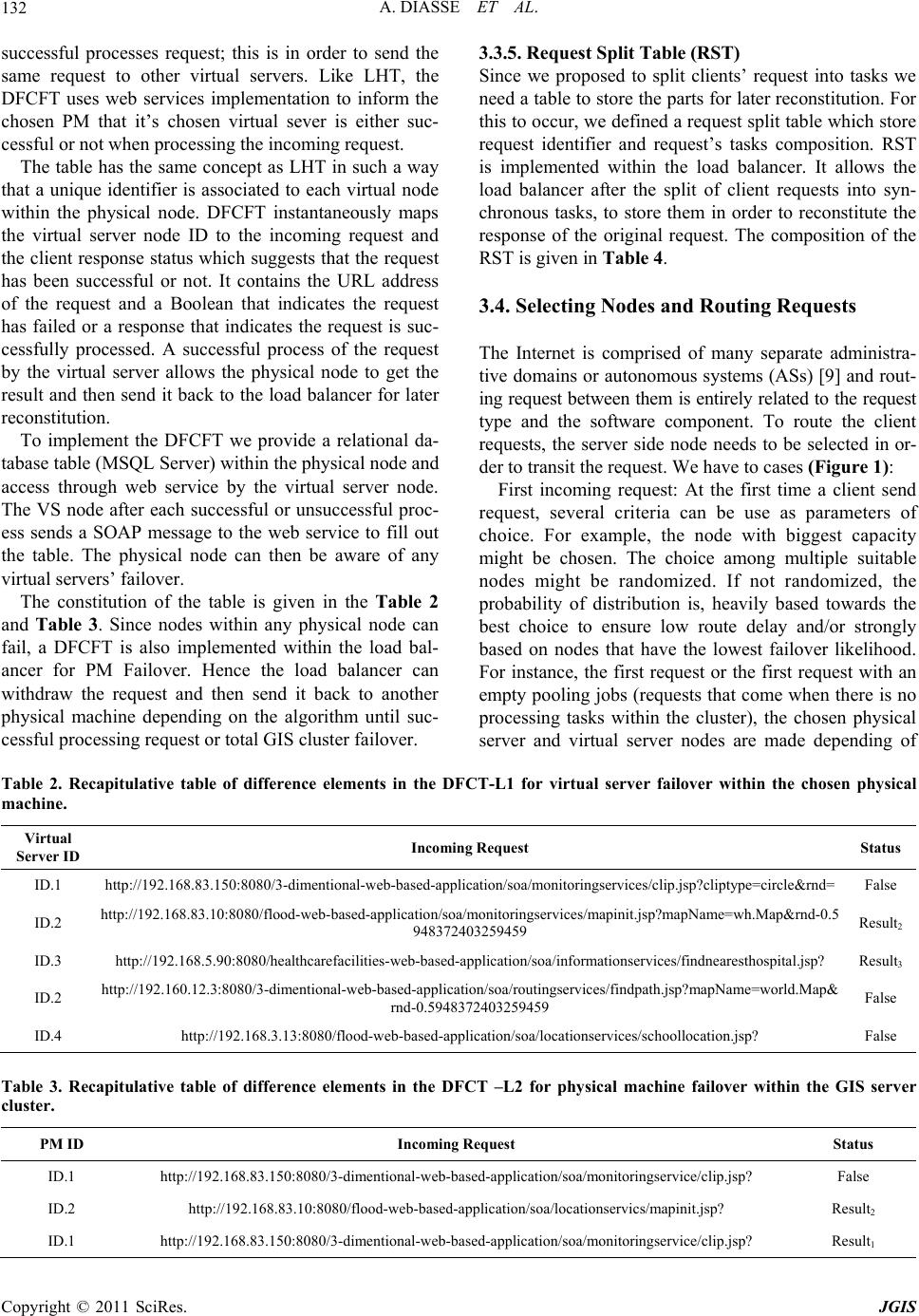

A. DIASSE ET AL. 132
successful processes request; this is in order to send the
same request to other virtual servers. Like LHT, the
DFCFT uses web services implementation to inform the
chosen PM that it’s chosen virtual sever is either suc-
cessful or not when processing the incoming request.
The table has the same concept as LHT in such a way
that a unique identifier is associated to each virtual node
within the physical node. DFCFT instantaneously maps
the virtual server node ID to the incoming request and
the client response status which suggests that the request
has been successful or not. It contains the URL address
of the request and a Boolean that indicates the request
has failed or a response that indicates the request is suc-
cessfully processed. A successful process of the request
by the virtual server allows the physical node to get the
result and then send it back to the load balancer for later
reconstitution.
To implement the DFCFT we provide a relational da-
tabase table (MSQL Server) within the physical node and
access through web service by the virtual server node.
The VS node after each successful or unsuccessful proc-
ess sends a SOAP message to the web service to fill out
the table. The physical node can then be aware of any
virtual servers’ failover.
The constitution of the table is given in the Table 2
and Table 3. Since nodes within any physical node can
fail, a DFCFT is also implemented within the load bal-
ancer for PM Failover. Hence the load balancer can
withdraw the request and then send it back to another
physical machine depending on the algorithm until suc-
cessful processing request or total GIS cluster failover.
3.3.5. Request Split Table (RST)
Since we proposed to split clients’ request into tasks we
need a table to store the parts for later reconstitution. For
this to occur, we defined a request split table which store
request identifier and request’s tasks composition. RST
is implemented within the load balancer. It allows the
load balancer after the split of client requests into syn-
chronous tasks, to store them in order to reconstitute the
response of the original request. The composition of the
RST is given in Table 4.
3.4. Selecting Nodes and Routing Requests
The Internet is comprised of many separate administra-
tive domains or autonomous systems (ASs) [9] and rout-
ing request between them is entirely related to the request
type and the software component. To route the client
requests, the server side node needs to be selected in or-
der to transit the request. We have to cases (Figure 1):
First incoming request: At the first time a client send
request, several criteria can be use as parameters of
choice. For example, the node with biggest capacity
might be chosen. The choice among multiple suitable
nodes might be randomized. If not randomized, the
probability of distribution is, heavily based towards the
best choice to ensure low route delay and/or strongly
based on nodes that have the lowest failover likelihood.
For instance, the first request or the first request with an
empty pooling jobs (requests that come when there is no
processing tasks within the cluster), the chosen physical
server and virtual server nodes are made depending of
Table 2. Recapitulative table of difference elements in the DFCT-L1 for virtual server failover within the chosen physical
machine.
Virtual
Server ID Incoming Request Status
ID.1 http://192.168.83.150:8080/3-dimentional-web-based-application/soa/monitoringservices/clip.jsp?cliptype=circle&rnd=False
ID.2 http://192.168.83.10:8080/flood-web-based-application/soa/monitoringservices/mapinit.jsp?mapName=wh.Map&rnd-0.5
948372403259459 Result2
ID.3 http://192.168.5.90:8080/healthcarefacilities-web-based-application/soa/informationservices/findnearesthospital.jsp? Result3
ID.2 http://192.160.12.3:8080/3-dimentional-web-based-application/soa/routingservices/findpath.jsp?mapName=world.Map&
rnd-0.5948372403259459 False
ID.4 http://192.168.3.13:8080/flood-web-based-application/soa/locationservices/schoollocation.jsp? False
Table 3. Recapitulative table of difference elements in the DFCT –L2 for physical machine failover within the GIS server
cluster.
PM ID Incoming Request Status
ID.1 http://192.168.83.150:8080/3-dimentional-web-based-application/soa/monitoringservice/clip.jsp? False
ID.2 http://192.168.83.10:8080/flood-web-based-application/soa/locationservics/mapinit.jsp? Result2
ID.1 http://192.168.83.150:8080/3-dimentional-web-based-application/soa/monitoringservice/clip.jsp? Result1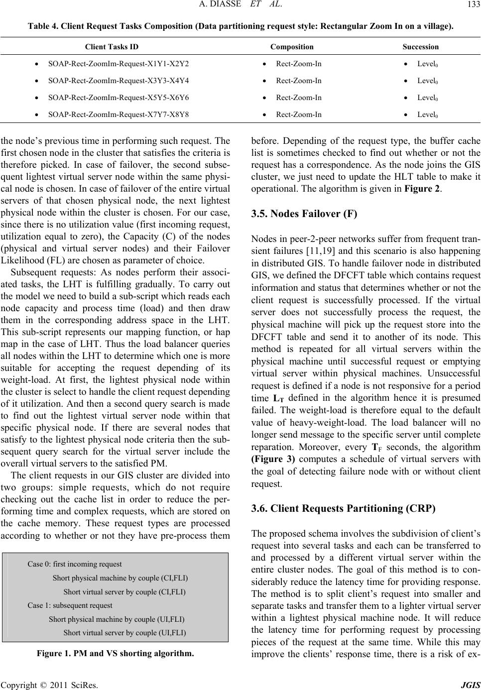

A. DIASSE ET AL.133
Table 4. Client Request Tasks Composition (Data partitioning request style: Rectangular Zoom In on a village).
Client Tasks ID Composition Succession
 SOAP-Rect-ZoomIm-Request-X1Y1-X2Y2  Rect-Zoom-In  Level0
 SOAP-Rect-ZoomIm-Request-X3Y3-X4Y4  Rect-Zoom-In  Level0
 SOAP-Rect-ZoomIm-Request-X5Y5-X6Y6  Rect-Zoom-In  Level0
 SOAP-Rect-ZoomIm-Request-X7Y7-X8Y8  Rect-Zoom-In  Level0
the node’s previous time in performing such request. The
first chosen node in the cluster that satisfies the criteria is
therefore picked. In case of failover, the second subse-
quent lightest virtual server node within the same physi-
cal node is chosen. In case of failover of the entire virtual
servers of that chosen physical node, the next lightest
physical node within the cluster is chosen. For our case,
since there is no utilization value (first incoming request,
utilization equal to zero), the Capacity (C) of the nodes
(physical and virtual server nodes) and their Failover
Likelihood (FL) are chosen as parameter of choice.
Subsequent requests: As nodes perform their associ-
ated tasks, the LHT is fulfilling gradually. To carry out
the model we need to build a sub-script which reads each
node capacity and process time (load) and then draw
them in the corresponding address space in the LHT.
This sub-script represents our mapping function, or hap
map in the case of LHT. Thus the load balancer queries
all nodes within the LHT to determine which one is more
suitable for accepting the request depending of its
weight-load. At first, the lightest physical node within
the cluster is select to handle the client request depending
of it utilization. And then a second query search is made
to find out the lightest virtual server node within that
specific physical node. If there are several nodes that
satisfy to the lightest physical node criteria then the sub-
sequent query search for the virtual server include the
overall virtual servers to the satisfied PM.
The client requests in our GIS cluster are divided into
two groups: simple requests, which do not require
checking out the cache list in order to reduce the per-
forming time and complex requests, which are stored on
the cache memory. These request types are processed
according to whether or not they have pre-process them
Case 0: first incoming request
Short physical machine by couple (CI,FLI)
Short virtual server by couple (CI,FLI)
Case 1: subsequent request
Short physical machine by couple (UI,FLI)
Short virtual server by couple (UI,FLI)
Figure 1. PM and VS shorting algorithm.
before. Depending of the request type, the buffer cache
list is sometimes checked to find out whether or not the
request has a correspondence. As the node joins the GIS
cluster, we just need to update the HLT table to make it
operational. The algorithm is given in Figure 2.
3.5. Nodes Failover (F)
Nodes in peer-2-peer networks suffer from frequent tran-
sient failures [11,19] and this scenario is also happening
in distributed GIS. To handle failover node in distributed
GIS, we defined the DFCFT table which contains request
information and status that determines whether or not the
client request is successfully processed. If the virtual
server does not successfully process the request, the
physical machine will pick up the request store into the
DFCFT table and send it to another of its node. This
method is repeated for all virtual servers within the
physical machine until successful request or emptying
virtual server within physical machines. Unsuccessful
request is defined if a node is not responsive for a period
time LT defined in the algorithm hence it is presumed
failed. The weight-load is therefore equal to the default
value of heavy-weight-load. The load balancer will no
longer send message to the specific server until complete
reparation. Moreover, every TF seconds, the algorithm
(Figure 3) computes a schedule of virtual servers with
the goal of detecting failure node with or without client
request.
3.6. Client Requests Partitioning (CRP)
The proposed schema involves the subdivision of client’s
request into several tasks and each can be transferred to
and processed by a different virtual server within the
entire cluster nodes. The goal of this method is to con-
siderably reduce the latency time for providing response.
The method is to split client’s request into smaller and
separate tasks and transfer them to a lighter virtual server
within a lightest physical machine node. It will reduce
the latency time for performing request by processing
pieces of the request at the same time. While this may
improve the clients’ response time, there is a risk of ex-

A. DIASSE ET AL. 134
Shorted PM cluster
Shorted VS cluster within physical machine
JIncoming = ΣTI where I in [0,n]
For T
I in JIncoming where TI
TIncoming = T
I
VS-appropriate = VS-0 [ PN-0]
VS-appropriate  TIncoming
Endfor
EndFunction
Figure 2. PM and VS selection algorithm.
LT is the latency time for performing such request
If ((R
T < LT) or (RT = LT)) then
TIncoming ---------not successful
VS-appropriate --------has fail
If (vs in pm is not finished)
VS-appropriate  VS-appropriate .Next
Else (vs in pm finished)
PM-appropriate  PM-appropriate .Next
VS-appropriate = PM-appropriate[0]
Endif
Else
TIncoming ----------successful
Endif
Figure 3. Load balancing system failover.
cessively fragmenting users’ request. An increasing
number of tasks would imply an augmentation in the
overlay hop length and size of routing and processing.
However the advantages provided by this method out-
weigh by far its disadvantages. Hence the number of
fragments must be optimized depending of the request.
However before dividing users’ request into several tasks,
we need to understand how request is being process
within such systems.
Without any similar techniques, client sends request to
the next tiers which are web server through the internet,
GIS services through SAOP messages over HTTP, load
balancing layer through HTTP protocol. In that latter
layer, load balancer uses the algorithm and sends the
request to a specific virtual server and after processing,
the response is sent back to the client interface through
the same path. Within the GIS virtual server, the client
request constituted several functions processed subse-
quently, depending on the input values and computer
memory space available. Even though there are set of
functions that can be processed at the same time, the
CPU processes the functions one by one, hence increase
response time.
In case of splitting clients’ request into synchronous
and equal tasks, they can be processed at the same time
in different GIS virtual servers and hence decrease re-
sponse time leading to high responsiveness. We pro-
posed to divide users’ requests into two types in our
D-GIS.
The first one is the request process as they are sending
without any modification of the inputs. These requests
are called the no-spitted requests. The second is the re-
quest that may split the input map into several pieces and
process the task on each piece on different virtual GIS
servers provided by the load balancing algorithm. For
instance when a client request a zoom-in on a portion of
the map, the latter can be divided into several equal maps
and each part will be applied to the client request using a
different virtual GIS server: Data Partitioning Request
Style (see equation (A) in Figure 4). This method is
mostly used to decompose simple GIS analysis functions.
However some functions cannot be split using this
method due to their implementation within the GIS serv-
ers. For instance the circle incoming map required a
clip-by-circle function can not be divided due to the
high-impossibility to decompose circle map into circular
map pieces.
Case example: In the case of request that allow the
client to select an interesting set of data for further in-
formation, the Data Partitioning Request Style is used on
the incoming square of map. For that matter the request
may be divided into four main tasks which are sending to
four different GIS servers depending of the load balanc-
ing handler or manager. The client request is send to the
web server which uses a software component to split the
incoming map into four rectangular boundary maps. The
four synchronous tasks are therefore performed by four
different GIS servers and the result is sent back to the
web server which replies to the request by displaying the
four ranges of maps. By performing the synchronous
tasks at the same time, the client response time is con-
siderably reduced.
3.7. Method Type Decomposition
Before decomposing the incoming request, the system
needs to identify the type of client request. Since we
proposed to subdivided clients’ requests into tasks and
send them to different GIS servers, we need a technique
to split request and store request’s task composition and
Jincoming = ∑ JI, where 1< I < {3, 5, 6} depending
of the scale level
(
Local
,
national and international
)
Figure 4. Equation A, data partitioning request style.

A. DIASSE ET AL.135
later reconstitute the response to the divided request to
send back to client interface. For implementing this
method, several critical issues must be discussed.
How can the incoming request be split? Where can the
client request (Client side or server side) be split? Which
device is responsible of the split (load balancer or spe-
cific engine)? How can the client request be split to re-
constitute meaningful processing tasks? How can the
device responsible for request split recognize data parti-
tion request style and no-partitioning request? Does the
client’s incoming request contain all information needed
to split the request? How can we have quasi-equal proc-
essing time in the different virtual server? To surrender
for an efficient load balancing, we suggest that:
The load balancer is responsible for client’s request
split. A request can either be split or not. If a split is used,
the request is a data partitioning request. Load balancer
identifies data partition request style depending on the
request input values. It can also identify, depending of
the client request URL, the GIS functions the server need
to call in order to process client’s request.
The load balancer also contains a file that determines
for each incoming client request the split method by
identifying the method type of the latter request.
Depending of our split method, the overall input map
is divided into twelve equal tasks. Each task from TI1 to
TI12 has quasi-equal processing time. The following
tables (Table 5 and Table 6) show the different splitting
tasks. The first table, even though it brings better per-
formance, may not be efficient due to the latency time
for getting every response for reconstitution. If the split
is not efficient we may be confront. However when split-
ting request into- quasi response time request, high per-
formance can be achieve.
When working on the algorithm (Figure 5) we en-
counter several problems two of which are as follows.
Problems 1: To get sophisticated performance when
balancing clients’ request, we try to solve an important
issue of load balancing which is persistent that is, where
to store the information about the client requests so sub-
sequent related-requests can be retrieve directly without
performing the same process?
Problems 2: One critical issue must be discussing the
balancing of client request into this cluster server. The
issue is that each request that enters the system has an
associate item which is composed of its popularity and
the amount of processing time it needs to be served to a
specific server or amount of serving time.
Problems 3: The decomposition of the request varies
depending of the input area. Splitting for example the
input query area into equal squares may not be efficient
for performing tasks. Hence split is done depending of
the quantity of information the input area contains: Quan-
tity of Information (QoI).
JIncoming --------the incoming job
Case 0: J
Incoming in No-partitioning
J
Incoming == JIncoming
Case 1: J
Incoming- in data partitioning
J
Incoming = ∑TIa’
where T
Ia’ are request tasks composition
depending of the input area quantity
of information
and 0 < Ia’ < N
Figure 5. Client split request algorithm method.
Table 5. Table of the input area split map (equal range).
TI1TI5TI9
TI2TI6TI10
TI3TI7TI11
TI4TI8TI12
Table 6. Table of the input area split map depending of the
quantity of information.
TI11TI1 TI2TI3TI8
TI5TI12TI7
TI10
TI6TI4TI1
3.8. Dynamic Distributed Load Balancing
Architecture
Our Dynamic Distributed Load Balancing architecture is
composed essentially of four elements: Load Balancers,
Load Algorithm, DFCFT and a LHT. The Load Balancer
which is a single server between the GIS servers cluster
and the GIS services cluster receives the client request
from the web server. Our design proposed the use of two
load balancers in case the first load balancer fails. The
secondary load balancer is configured to take over the
client request balancing to provide high availability of
the system. Load Algorithm control the selecting of
physical and virtual server nodes, write information onto
the LHT and DFCFT. The DFCFT controls the system
failover by sending back the request to the physical node
in order for the latter to redirect it to another virtual
server. At last we have, the LHT, controlled by the load
algorithm. The distributed dynamic load balancing ar-
chitecture is given in the following figure (Figure 6).
3.9. Dynamic Distributed Load Balancing
Algorithm
Since it is very hard to address the load balancing prob-

A. DIASSE ET AL. 136
Figure 6. Dynamic & distributed load balancing general architecture in distributed GIS.
Table 7. Definition of some parameters formula.
Ui =Wi/Ci Machine I = ∑ VSIa where 1 < a < n
W
i if W i < Ci
RTSP = Ci if W
i > Ci
0 if node fail
Wi = ∑ Wvsⁿ
where vs №1 < vsⁿ < vs №n
FL =RTSP / NJobsAssigned
where NJobsAssigned is the number of jobs send to node
lem in its full generality, we make some simplifying as-
sumptions, which we believe are reasonable in practice
for a distributed-based GIS application. Some symbolo-
gies used are also presented in Table 7.
 A job J is a task in the split request table and must
run contiguously on one machine.
 Arrived job J sent to node I may be processed by
the node itself
 It may be transferred to another node if there is
failover.
 Each node I has N virtual servers VSI named VSI1,
VSI2, VSI3…SIn which we limit to 3.
 The Ci is the capacity of the physical node I and
Cvsia is it virtual server a, which is related to for
example, available disk space, processor speed, or
bandwidth.
 A node’s utilization Ui is the fraction of its capac-
ity Ci and it load Wi [8] and [12].
 Finally each virtual server can process at least one
job at a time.
We consider that the associate item is equal for each
incoming request. Then they are negligible for the pur-
pose of this study.
We decided for the purpose of the model to keep client
information in the web server layer for an efficient load
balancing.
4. DDLB Prototype Design
D-GIS is defined as the use of internet technologies to
distribute geographic information in a variety of forms,
including maps, images, datasets, spatial analysis opera-
tions and reports. It is an advanced model which com-
bines both an advancement of internet GIS and Mobile
GIS advanced models. The distributed GIS encounter the
most complete GIS system and embed Mobile GISs and
Web-GIS. Its architecture is therefore as general as pos-
sible. The next figure will present the prototype design
proposed in this paper. This design will focus of the sys-
tem layering model and particularly of the two load bal-
ancing layers (Figure 8).
By incorporating the Network Load Balancing and the
Dynamic Distributed Load Balancing model into our
distributed GIS, we obtain the overall system schema
which provides high performance and responsiveness
distributed GIS application. The schema is composed of
five system tiers (client tier, web server tier, GIS web
services tiers, GIS servers tier and spatial data servers
tier) and two algorithm layer models.
5. Result and Discussion
For assuring the effectiveness of our method, we provide
a simulation that shows satisfaction. Although the pro-
posed algorithm is quiet long (Figure 7), it simplicity and
speed allows the load balancing to deliver very high per-
formance, including both high throughput and low res-
ponse time, in a wide range of useful GIS applications. For
example when one web-based GIS client requests for a

A. DIASSE ET AL.137
Step 0: update LHT nodes after assignation
Step 1: Select the load balancer use to dispatch client’s requests into cluster servers
If (LBPrimary working )
Step 2: Loop all Jobs send to the load balancer handler
Step 3: split the incoming request into synchronous and asynchronous tasks
Step 4: Open the LHT and get the information about each virtual server
Step 5: call the shorting function to range PM and its VS from lightest to heaviest
Step 6: Select appropriated VS of appropriate PM and assign synchronous tasks
Step 7: task being process by the chosen virtual server within the chosen PM
Step 8: call the failover function to find out whether task fails or not
Step 9: select the next incoming job
Figure 7. Dynsmic distributed load balancing algorithm.
Table 8. MapGIS K9 server-based response time before and after load balancing (millisecond).
Characteristics Map Request Response Time MapGIS-K9 IMS
No web caching Time per Map at launch time 54000
Time per map to access for displaying vector map 5500
Time per map to access for displaying tile map 600 1 client on 1 GIS server
Time per map to individual access for query 4300
Average time for simultaneous displaying 16300
Time per map to access for displaying tile map 945
4 clients on 1 GIS server
Average time for simultaneous query 12690
Average time for simultaneous displaying vector 4530
Average time for simultaneous displaying tile map 1165
45 clients on 4 GIS server
Average time for simultaneous query 4396
Average time for simultaneous displaying vector 3482
Average time for simultaneous displaying tile map 963
45 clients on 5 virtual
GIS servers
Average time for simultaneous query 3836
query operation, the web server receives spatial query
request from loading the web page through the client
web browser. The load balancer receives the spatial
query from the web server, partitions the input region
into uniform tile-based regions using spatial operation,
assigns the partitioned regions to several GIS servers,
allows one GIS server to process queries for a certain
region, and dynamically reallocate GIS servers for proc-
essing the queries by receiving each GIS server query
processing response of it regions.
By calling map initialization, query processing, select
regions functions into the distributed application, the
client response time is highly reduced. The GIS server
setups on virtual servers are therefore preventing the
concentration of work on the system.
We show that unlike previous methods of providing
high performance and responsiveness in distributed GIS,
our model is tied to the number of virtual servers used,
their capacity and frequency of failover and consequently
provide high performance load balancing. Yet, the model
can handle the heterogeneity of a distributed GIS system,
system failover of virtual servers and physical machines,
and high scalability to meet future need. We can see in
Table 8 that the response time for an individual query
task before applying solution (4300) are almost the same
as the response time for simultaneous query task on a
cluster GIS server (4396).
6. Conclusions and Future Works
The aim of the work was to provide solution for high
performance and responiveness distributed GIS s

A. DIASSE ET AL. 138
Figure 8. Dynamic & distributed-based load balancing general configuration in distributed GIS system.
in order to overcome distributed GIS problems which are
encountered on the rapidity of distributed GIS applica-
tions. Several methods and techniques have been intro-
duced for that matter but few researches were focused on
load balancing in GIS system. By incorporating a Dy-
namic Distributed load balancing model into our distrib-
uted GIS, we obtain the overall schema which enhances
GIS application effectiveness.
The performance carries out the action or accom-
plishes of task, especially the one requiring care or skill
[9]. It is defined as the possibility of optimizing, which is
the enhancement of effectiveness and is related directly
to the execution time of the computers in which the task
is being processed and depended on the interfaces be-
tween the processor and the memory.
In D-GIS, the performance of application is an over-
whelming issue since rendering the combination of huge
data and information, multiple simultaneous clients’ re-
quests and cross processes and platforms call from client
to server brings down the latency time to provide re-
sponses. Our solution provides high scalability, high
availability, and good load balancing capabilities; hence
GIS system organization can increase their business
force by making clients happy to use their software.
7. Acknowledgements
The work is supported by National "863" plan: Research
and software development of three-dimensional spatial
information service technique of the network
(No.2009AA12Z211).
8. References
[1] S. Malik, “Dynamic Load Balancing in a Network of
Workstation,” 95.515 Research Report, 19 November,
2000.
[2] Sandeep Sharma, Sarabjit Singh, and Meenakshi Shar-
ma, “Performance Analysis of Load Balancing Algo-
rithms,” Proceedings of World Academy of Science, En-
gineering and Technology, Vol. 38, 2008.
[3] Y. R. Lan, “A Dynamic Load Balancing Mechanism for
Distributed Systems,” Journal of Computer Science and
Technology, Vol. 11, No. 3, 1996, pp. 192-207.
[4] A. Sayer, “Thesis Proposal: High Performance, Federa-
tion and Service-Oriented Geographic Information Sys-

A. DIASSE ET AL.139
tems,” Indiana university, Indiana.
[5] P. S. Zhao and C. J. Yang, “The Study on the Architec-
ture of Web-GIS by Institute of RS Applications,” Chi-
nese Academy of Sciences,Beijing.
[6] D. L. Eager, E. D. Lazowska and John Zahorjan, “Adap-
tive Load Sharing in Homogeneous Distributed Systems,”
IEEE Transactions on Software Engineering, Vol. 12, No.
5, May 1986, pp. 662-675.
[7] A. Sharma, S. Singh, and Meenakshi, “Sharma: Per-
formance Analysis of Load Balancing Algorithms,” Pro-
ceedings of World Academy of Science, Engineering and
Technology, Vol. 38, 2008.
http://masters.donntu.edu.ua/2010/fknt/babkin/li-
brary/article11.pdf
[8] B. Godfrey, K. Lakshminarayanan, S. Surana, R. Karp
and I. Stoica, “Load Balancing in Dynamic Structured
P2P Systems,” Performance Evaluation, Vol. 63, No. 3,
2006, pp. 217-240.
http://www.ieee-infocom.org/2004/Papers/46_4.PDF
[9] J. Feigenbaum and S. Shenker, “Distributed Algorithmic
Mechanism Design Recent Results and Future Direc-
tions,” DIALM '02 Proceedings of the 6th international
workshop on Discrete algorithms and methods for mobile
computing and communications, New York, 2002.
[10] T. Horanont, N. K. Tripathi and R. Raghavan, “A Com-
parative Asseessment of Internet GIS Server systems,”
Space Technology Applications and Research Program,
School of Advanced Technologies Asian Institute of
Technology, Thailand, 2005.
[11] W. J. Bolosky, J. R. Douceur, D. Ely and M. Theimer,
“Feasibility of a Serverless Distributed File System an
Existing Set of Desktop PCs,” Proceedings of the de-
ployed on International Conference on Measurement and
Modeling of Computer Systems, Santa Clara, CA, June
2000, pp. 34-43.
[12] J. Ledlie and M. Seltzer, “Distributed, Secure Load Bal-
ancing with Skew, Heterogeneity, and Churn,” Division
of Engineering and Applied Science, Harvard University,
September 2009.
http://dash.harvard.edu/bitstream/handle/1/2962660/Seltz
er_DistributedSecure.pdf?sequence=2
[13] P. B. Godfrey and I. Stoica , “Heterogeneity and Load
Balance in Distributed Hash Tables,” Computer Science
Division, University of California, Berkeley.
[14] D. R. Karger and M. Ruhl, “Simple Efficient Load Bal-
ancing Algorithm for Peer-to-Peer Systems,” SPAA '04
Proceedings of the sixteenth annual ACM symposium on
Parallelism in algorithms and architectures, 2004.
http://static.googleusercontent.com/external_content/un-
trusted_dlcp/research.google.com/fr//pubs/archive/33339.
pdf
[15] A. Rao, K. Lakshminarayanan, S. Surana, R. Karp and I.
Stoica, “Load Balancing in Structured P2P Systems,”
Proceedings of IEEE INFOCOM, February, 2003.
http://www.ieee-infocom.org/2004/Papers/46_4.PDF
[16] F. Dabek, M. F. Kaashoek, D. Karger, R. Morris and I.
Stoica, “Wide-area Cooperative Storage with CFS,”
SOSP '01 Proceedings of the eighteenth ACM symposium
on Operating systems principles, Vol. 35, No. 5, pp.
202-215.
[17] Hash Table from Wikipedia the Free Encyclopaedia,
Access on April 2010.
http://en.wikipedia.org/wiki/Hash_table
[18] Virtual Server form Wikipedia.
http://en.wikipedia.org/wiki/Virtual_private_server
[19] L. P. Cox and B. D. Noble, “Samsara: Honor among
Thieves in Peer-to-Peer Storage,” Department of Electri-
cal Engineering and Computer Science, University of
Michigan Ann Arbor, MI 48109-2122. Page 4.
http://www.eecs.harvard.edu/~mema/courses/cs264/paper
s/samsara-sosp2003.pdf