 Int. J. Communications, Network and System Sciences, 2011, 4, 241-248 doi:10.4236/ijcns.2011.44029 Published Online April 2011 (http://www.SciRP.org/journal/ijcns) Copyright © 2011 SciRes. IJCNS Active Queue Management within Large-Scale Wired Networks Ping-Min Hsu1, Chun-Liang Lin1, Ching-Han Yu2 1Department of Electrical Engineering, National Chung Hsing University, Taichung, Chinese Tai pei 2Department of Electrical Engineering, National Taiwan University, Chinese Taipei E-mail: chunlin@dragon.nchu.edu.tw Received March 3, 2011; revised March 24, 2011; accepted March 30, 2011 Abstract Signal transmission control protocol sources with the objective of managing queue utilization and delay is actually a feedback control problem in active queue management (AQM) core routers. This paper extends AQM control design for single network systems to large-scale wired network systems with time delays at each communication channel. A system model consisted of several local networks is first constructed. The stability condition guaranteeing overall stability is subsequently derived using Lyapunov stability theory. The results developed have been successfully verified on a network simulator. Keywords: Large-Scale System, Network Control, Stability, Time Delay 1. Introduction Traffic characterization and modeling are generally rec- ognized as two important steps toward analysis and con- trol of network transmission performance. With the aid of the characterized model, control theory can be effi- ciently applied in solving the congestion control problem. There have been various delayed differential equation models developed in [1-3], in which the fluid-flow model utilized in [1] was previously proposed in [2]. Those characterized data traffic as fluid used a set of differen- tial equations to describe the Active Queue Management (AQM) policy and the router queuing process. In [4], the end-to-end congestion control mechanisms were em- ployed in transmission control protocol (TCP) flow con- trol. While a bunch of research focusing on modeling and analysis of network control systems have been published, most approaches addressed the issue for a single sender- receiver network connection [5]. This paper is motivated by the requirement of an ap- proach for modeling and stabilization of large-scale communication networks. An extension of the fluid- based model in wireless networks was proposed in [6,7], in which their parameters for representing the probability of data transmission failure was applied in system de- velopment. A system for mixed wired and wireless net- works was concerned in [6], in which a more general fluid-based model compared with that in [1] was pro- posed. A robust controller design was proposed in [7], in which the stability analysis was conducted by Lyapunov theory and modern control theory was ex- tended to deal with the network congestion problem. Fur- thermore, linear matrix inequalities were proposed in control design and less oscillation under TCP was achieved. Packet dropout not only affects stability in data transmission, but also plays an important role in the net- work control systems. The authors in [8-10] have inves- tigated stability for the network control systems with packet dropout. To the best of the authors’ knowledge, while the Lya- punov stability theory has been widely applied to the stability analysis of large-scale systems [11-13], investi- gation for stability of the large-scale network control systems (LWNCSs) are quite rare. This motivates this research. The presented work shows that an appropriate control design based on an appropriate Lyapunov func- tional ensuring asymptotic stability of the LWNCS can be constructed when there are a large number of signal flows. The major contributions can be summarized as fol- lows. 1) A control strategy for congestion control in the large-scale wired network is constructed. 2) All local networks are interconnected according to the dropping probability. That is, how the local net- 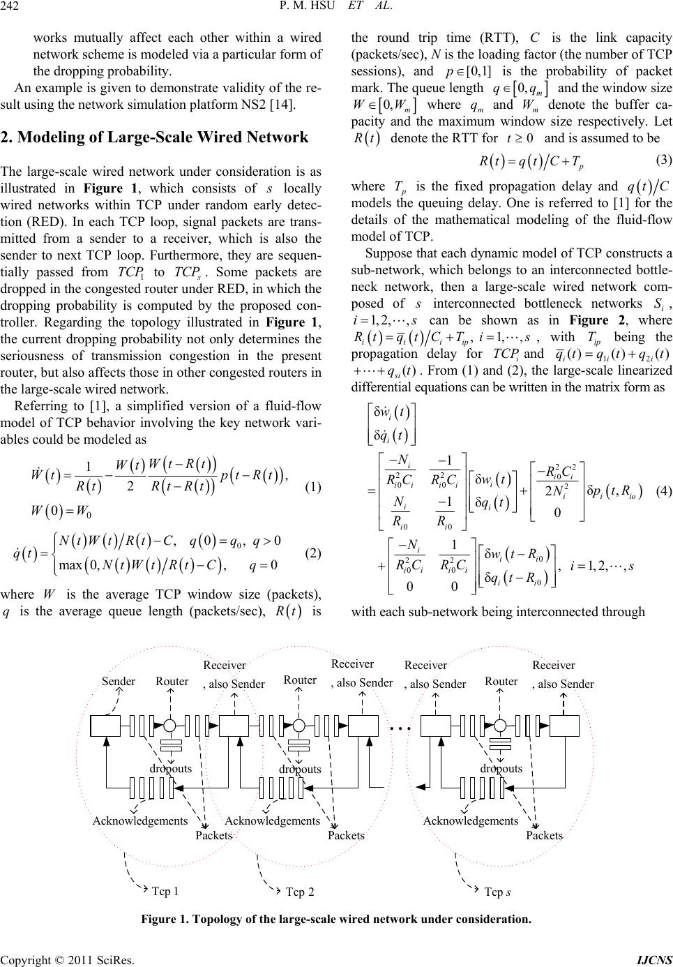 P. M. HSU ET AL. 242 works mutually affect each other within a wired network scheme is modeled via a particular form of the dropping probability. An example is given to demonstrate validity of the re- sult using the network simulation platform NS2 [14]. 2. Modeling of Large-Scale Wired Network The large-scale wired network under consideration is as illustrated in Figure 1, which consists of locally wired networks within TCP under random early detec- tion (RED). In each TCP loop, signal packets are trans- mitted from a sender to a receiver, which is also the sender to next TCP loop. Furthermore, they are sequen- tially passed from 1 TC to P TCP. Some packets are dropped in the congested router under RED, in which the dropping probability is computed by the proposed con- troller. Regarding the topology illustrated in Figure 1, the current dropping probability not only determines the seriousness of transmission congestion in the present router, but also affects those in other congested routers in the large-scale wired network. Referring to [1], a simplified version of a fluid-flow model of TCP behavior involving the key network vari- ables could be modeled as 0 1, 2 0 Wt Rt Wt Wtpt Rt Rt Rt Rt WW (1) 0 ,0, max0,, 0 NtWt RtCqqq qt NtWt RtCq 0 (2) where is the average TCP window size (packets), is the average queue length (packets/sec), W q Rt is the round trip time (RTT), is the link capacity (packets/sec), N is the loading factor (the number of TCP sessions), and C [0,1]p is the probability of packet mark. The queue length 0,qqm and the window size 0, m WW where m q and m W denote the buffer ca- pacity and the maximum window size respectively. Let Rt denote the RTT for and is assumed to be 0t Rtqt C T (3) where p is the fixed propagation delay and T qt C models the queuing delay. One is referred to [1] for the details of the mathematical modeling of the fluid-flow model of TCP. Suppose that each dynamic model of TCP constructs a sub-network, which belongs to an interconnected bottle- neck network, then a large-scale wired network com- posed of interconnected bottleneck networks i, S 1, 2,,is can be shown as in Figure 2, where , 1,, iiiip Rtqt CTis, with being the propagation delay for i TCP and ip T 12 () () ()q t iii si qt tq ()tq . From (1) and (2), the large-scale linearized differential equations can be written in the matrix form as 22 22 0 00 2 00 0 22 00 0 δ δ 1 δ δ, (4) 2 1δ 0 1δ , 1,2,, δ 00 i i i ii i ii iiiio i ii ii iii ii ii ii wt qt NRC wt RC RCptR N Nqt RR Nwt R RC RCis qt R with each sub-network being interconnected through Router Sender Receiver , also Sender Packets Acknowledgements Router Receiver , also Sender Router Receiver , also Sender Receiver , also Sender Tcp 1 Tcp 2Tcp Packets Acknowledgements Packets Acknowledgements dropouts dropouts dropout s Figure 1. Topology of the large-scale wired network under consideration. Copyright © 2011 SciRes. IJCNS  P. M. HSU ET AL. Copyright © 2011 SciRes. IJCNS 243 1 w 1 w 1 p 1 q 1 q 1 1 R 2 w 2 w 2 p 2 q 2 q 2 1 R TCP 1 TCP 2 1 2 w w p q q TCP routed packets data packets Congested Router 1 Congested Router 2 Congested Router s 11 q 1 q 12 q 2 q 1 q s q AQM control law AQM control law 1 2 1 2 1 1 2 1 1 s e 2 s e 1 1 R 1 C 2 C 1 N 2 N 2 1 R N C 1 R AQM control law s e 1 1 R 21 q 22 q 2 q Figure 2. Block diagram of the large-scale wired network. 0 0 0 0 1 0 01 0 333 0 0 233 0 δ,dδ δd 2δd 2δd,,1,2 i i i s iiopiijj ij j s ii piiji j R ii ii R ii ii R ptRKqqth pptvvKdt v NwtvvRC v NqtvvRCij v u ,s (5) where ij is the transmission time between the bottleneck networks i and hS S; , 0 δiii www δi q 0i qq , 0jj qqq , and 0; 00 0i denoting our operating point; i and δpp iii p i wq ,,p q q i N denote data packets belonging to the ith and jth sub-networks respectively; i denotes the ith expected TCP sending window; i denotes the link capacity; denotes the number of the ith TCP sessions; wC 00iiip RqC max p Tp; i is the probabil- ity of packet mark; RED consists of a proportional con- troller and packet-marking profile, shown as in Figure 3, where , and are configurable parame- ters and pi denotes the slope of the active queue management control law which computes i as the func- tion of the measured queue length mi qn K max q p i q by the AQM pol- icy; ij is the flow distribution ratio from the bottle- neck network d S to i. If S i qt is bounded by and , the packet-marking probability is given by min q max q 0 0 0 0 1 0 1 30 33 0 20 33 0 δ δdd 2 δd 2 δd i i i ipiijj ij j s ipiiji Rj ii R ii ii R ii pKdq qth pt vv Kt v Nwt vv v RC Nqt vv v RC u min qmax q max p i p 1 i q i p itu - + i q acket-marking profile Figure 3. RED drop function. The form of (5) is determined based on the following considerations. 1) While each sub-network is interconnected through (5), the feedback signal applied for the controller is treated as the combination of all the queue lengths in the large-scale network. Thus, the term 0 1δ s ijj ij jdq qth in (5) was claimed. It was further multiplied with i K, which denotes the slope of the active queue management control law. 2) The term 0 0δd ii R tvv v denotes the differ- ence between the current and delayed values of the dropping probability adopted in the ith TCP. Con- sidering the fluid-flow model, the current queue length variation is affected by the delayed dropping probability while the current one is applied in real world. Considering this fact, while constructing (5), the term 0 0δd ii R tvv v is added. 3) 0i p is added to cancel 0i p while computing where δ i p 0iii ppp . 4) Additional terms in the AQM controller law are added to obtain the transformed system (6) with the controller (7). 5) Now, substituting 0 δ, ii ptR, defined by (5), into (4) gives a new system. Based on (4), a large-scale wired network system consisting of s local net- works can be expressed in the state-space repre- sentation as follows , 1,2,, iiiiii ttti Ax Bus (6) where δδ T iii twtqt x, 2 0 00 2i N0 1 ii ii i ii RC N RR , 2 0 2 2 0 ii ii RC N B, and A 1 ()()(()), ,1,2,, s iijjijii j tFxth tij uus (7) with 0 ijpi ij d F and iii tKtux being the AQM control law for the ith subsystem, and  P. M. HSU ET AL. 244 0 0 0 00 1 0 30 33 0 20 33 0 δd 2 δd 2δd i i i iipi ijii j i R ii R ii ii R ii tKdq tp pt vv v Nwt vv vRC Nqtvv v RC uu Equation (6) represents the linearized system of the large-scale wired network while considering coupling effects induced by the locally wired networks. The term implies the dropping probability while concerning the interconnection of local networks. The term itu itu is to be determined in the stability analysis. Equation (7) is treated as the control input such that 0ii pttpui is applied as the dropping probability. itu can be derived in the following steps: Step 1) Consider (5), which models how local net- works may mutually affect each other in the large-scale wired networking environment. Step 2)Substitute 0 δ, ii ptR into (4) and use i x to obtain system of (6) with the controller (7). 0ii tRx From (6) it is easily seen that is controllable. The action of the AQM control law is to mark packets as a function of the measured queue length q. The plant dynamics given by (6) relates reveals the packet-marking probability dynamically affects the queue length. , ii i AB Now, let the set of feasible operating conditions 00, m qq, 00, i wWm , and 00,1 i p. Assume that , and are continuously differentiable δi wδiδi pq on 0, 0 i R, i.e. iW w b v , δiq qb v , δ ip pb v , 0, 0 i vR . Therefore 0 0 0 δd iiW Rwt vvbR v i , 0 0 0 δd iiq Rqt vvbR v i , 0 0 0 δd iip RptvvbR v i . Furthermore 2 0 11 0 ss iiipiijipi iji jj ii i ttKdtKqd pgtt uu uu u t (8) where 0 0 0 30 33 0 20 33 0 0 2δd 2δd +δd i i i i ii R ii ii R ii i R N twt vRC Nqt vv v RC pt vv v vv It is seen that im iim gt g with 3 23 0 2i im W ii N b RC 2 0 23 0 2iqip b ii NbR RC . The gain i K is chosen as 0 0 1 0 0 1 1,when 0, 1, 2,, 1, otherwise, iimi s ij j pi iim s ij j pg qd is pg qd u (9) This ensures 0, iii i ttuu ut. With regard to the above system one can ensure that i , 1, 2,,is satisfy 2, , 1,2,, iiiiii tt ttRis uu u u(10) From (8) and (9), the gain reduction tolerance is given by 1 s ipi jij d where are chosen ,1,, ij dj s 1 such that 1 s ip i ij j Kd . 3. Stability of LWNCS The following theorem states the main result which cha- racterizes the stability condition for the LWNCS. Lemma: For any scalar 0 and any real vectors and Y with appropriate dimension, then TTT 1 T YYX XXYY (11) Theorem: The large-scale wired network system de- scribed by (6), which satisfies (10), would be asymptoti- cally stable, if the state feedback control law of each sub-network is given by 1, 1,2,, 2 T iiiii tti uBPx s (12) where 1 iii with i satisfying 221 221 iiiii (13) and 0 T ii PP satisfies the following Riccati matrix inequality: TT 1 +1 0 ii ii iiiniii ii in s s PPA PIBBP I (14) Copyright © 2011 SciRes. IJCNS  P. M. HSU ET AL. Copyright © 2011 SciRes. IJCNS 245 in which 1 is a positive constant, 2 () iiii 4 and :max,1,2,, iji js with ji satisfying Proof: The stability analysis is derived around the ori- gin δδ0 ii qw of (4), i.e. the equilibrium point 000 ,, ii qpw of the fluid-flow model. Regarding the problem, we define an appropriate Lyapunov functional candidate as 1 1,, TT ij nijiiijij IFBBF (15) TT 2 0 0 11 dd ij ss tt t T iiiiiijjjiii i th ij tt 2 d Vxx Pxx xxxu(16) for . The set 1,2,,i s 000 ,, ii qpw chosen as the equilibrium point of the fluid-flow model corresponding to is determined by i TCP 2 00 00 00 000 10,0,, 1 2 ii iiiiipi ii ii wN q pwCRTp RR RC It is obtained that 00 iVwhile 0 i uand for . Taking differentiation with re- spect to time t and using (6) while ignoring and 0 ii xV0 ix T 100 s ii i xx 2 10 s i i u gives TT 1 22 T 11 T 1 TT 11 +2 +2 s iiiiiiiii ni i ss iiiiiij jij ii s iiiii i ss ijjjjijjij ij Vt It tt th tt ttth th xxAPPAx uxPBFx xPBu xx xx It is easily obtained from (11) that TTT T 11 TTT 11 1 T 1 TT 11 1 T 1 1 1 1 ss ijijiiii iiijj ij ij ss jijijiiijjij ij iiii ss T jijijiiijjij ij s iiii i tht tth th th tt th th stt xFBPxxPBFx xFBBFx xPPx xFBBFx xPPx T 1 TT 1 2 s iiiii i s ii iiiiii i tt tP xPBu xPBBxt (17) Furthermore TT 11 1 ss s ijjji ii ij i tts tt xx xx Therefore, it can be obtained that TT 2 1 1 2 TTT 11 1 1 1 +4 1 + s iiiiii iiiini i T ii iiiiiii ss ijijiiijijnjij ij tss t th th VxxAP PAIP PBB Px xFBBFIx where 10 . After substituting (12) into (10), one gets (18) TTT 2 iiiiiiii iiiii txt t xPBBP xPBut From (12)-(15), it can be concluded that i.e. T TT TT 1111 11 0 0 11 0,, i s ii ii iiiiiinisiiisisn J tt diag Vx FBBF IFBBF I (19) 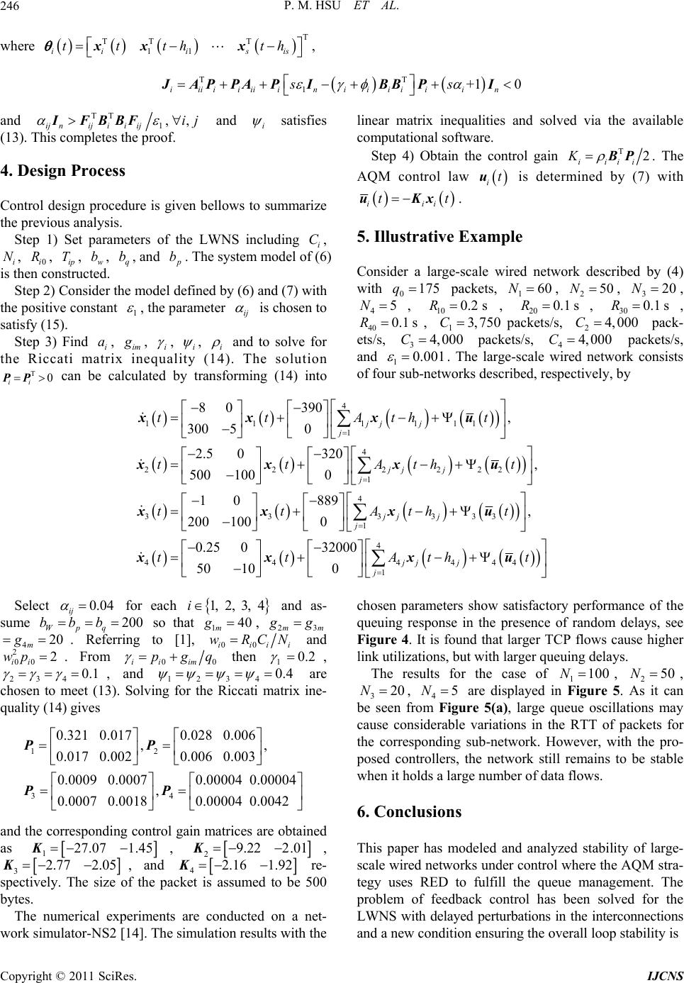 P. M. HSU ET AL. Copyright © 2011 SciRes. IJCNS 246 where , T TT T 11iii sis ttthth xx x TT 1+1 0 iiiiiiiiniiiiii n ss JAPPAPIBBPI and TT 1,, ij nijiiijij IFBBF and i satisfies (13). This completes the proof. 4. Design Process Control design procedure is given bellows to summarize the previous analysis. Step 1) Set parameters of the LWNS including i, i, 0i, ip, w, , and C N RTbq b b. The system model of (6) is then constructed. Step 2) Consider the model defined by (6) and (7) with the positive constant 1 , the parameter ij is chosen to satisfy (15). Step 3) Find i, im a , i , i , i and to solve for the Riccati matrix inequality (14). The solution can be calculated by transforming (14) into T0 ii PP linear matrix inequalities and solved via the available computational software. Step 4) Obtain the control gain T2 iiii K BP . The AQM control law itu is determined by (7) with iii tt uKx. 5. Illustrative Example Consider a large-scale wired network described by (4) with 0175q packets, , , 160N250N320N , 4 N5 , , 20 , , 40 , 10 R 0.1 sC0.2 s 13,750 0.1 sRR 30 0.1 s R packets/s, pack- ets/s, 24,C000 34, 0C00 packets/s, 4 packets/s, and 1 4, 000C 0.001 . The large-scale wired network consists of four sub-networks described, respectively, by 4 11 1111 1 4 22222 1 4 333333 1 4 80 390, 300 50 2.5 0320, 500 1000 10 889, 200 1000 0. jj j j jj j j jj j j ttAtht ttAth ttAth t 2 t t xx xu xxx xx xu x u 4 4444 1 25 032000 50 100jj j j tAth 4 t xxu Select 0.04 ij Wpq bbb for each and as- sume so that , 1, 2, 3, 4i 140 m g 20023mm g . Referring to [1], 4m g2000ii wRCi N i and . From 2 00 ii wp 200ii im qpg then , 234 1 0.2 0.1 , and 1234 0.4 are chosen to meet (13). Solving for the Riccati matrix ine- quality (14) gives 12 34 0.321 0.0170.028 0.006 , 0.017 0.0020.006 0.003 0.0009 0.00070.00004 0.00004 , 0.0007 0.00180.00004 0.0042 PP PP , and the corresponding control gain matrices are obtained as 127.07 1.45 K, 29.22 2.01 K, 3, and 2.77 2.05 K 42.16 1.92 K re- spectively. The size of the packet is assumed to be 500 bytes. The numerical experiments are conducted on a net- work simulator-NS2 [14]. The simulation results with the chosen parameters show satisfactory performance of the queuing response in the presence of random delays, see Figure 4. It is found that larger TCP flows cause higher link utilizations, but with larger queuing delays. The results for the case of 1, 2 100N50N , 320N , 45N are displayed in Figure 5. As it can be seen from Figure 5(a), large queue oscillations may cause considerable variations in the RTT of packets for the corresponding sub-network. However, with the pro- posed controllers, the network still remains to be stable when it holds a large number of data flows. 6. Conclusions This paper has modeled and analyzed stability of large- scale wired networks under control where the AQM stra- tegy uses RED to fulfill the queue management. The problem of feedback control has been solved for the LWNS with delayed perturbations in the interconnections and a new condition ensuring the overall loop stability is  P. M. HSU ET AL.247 (a) (b) (c) (d) Figure 4. Transient response of queueing with 160N , 2, 3 50N20 and 4. (a) Queue size for TCP1; (b) Queue size for TCP2; (c) Queue size for TCP3; (d) Queue size for TCP4. 5N (a) (b) (c) (d) Figure 5. Transient response of queueing with 1100N , 250N , 320N and 45N . (a) Queue size for TCP1, (b) Queue size for TCP2; (c) Queue size for TCP3; (d) Queue size for TCP4. Copyright © 2011 SciRes. IJCNS  P. M. HSU ET AL. Copyright © 2011 SciRes. IJCNS 248 presented. The simulation study conducted on the NS2 has been verified successfully. 7. Acknowledgements This research was sponsored by National Science Council, Taiwan under the grant NSC No. 95-2221-E-005-017. 8. References [1] C. V. Hollot, V. Misra, D. Towsley and W. B. Gong, “Analysis and Design of Controllers for AQM Routers Supporting TCP Flows,” IEEE Transactions on Auto- matic Control, Vol. 47, No. 6, 2002, pp. 945-959. doi:10.1109/TAC.2002.1008360 [2] V. Misra, W. B. Gong and D. Towsley, “Fluid-Based Analysis of a Network of AQM Routers Supporting TCP Flows with an Application to RED,” Proceedings of ACM Special Interest Group on Data Communication, Stock- holm, 28 August-2 September 2000, pp. 151-160. [3] P. F. Quet and H. Ozbay, “On the Design of AQM Sup- porting TCP Flows Using Robust Control Theory,” IEEE Transactions on Automatic Control, Vol. 49, No. 6, 2004, pp. 1031-1036. doi:10.1109/TAC.2004.829643 [4] B. A. Chiera and L. B. White, “A Subspace Predictive Controller for End-to-End TCP Congestion Control,” Proceedings of Australian Communications Theory Work- shop, Brisbane, 2-4 February 2005, pp. 42-48. doi:10.1109/AUSCTW.2005.1624224 [5] S. Tarbouriech, C. T. Abdallah and J. Chiasson, “Ad- vances in Communication Control Networks,” Springer, Berlin, 2005. [6] K. Zhang and C. P. Fu, “Dynamics Analysis of TCP Ve- no with RED,” Computer Communications, Vol. 30, No. 18, 2007, pp. 3778-3786. doi:10.1016/j.comcom.2007.09.004 [7] F. Zheng and J. Nelson, “An H∞ Approach to Congestion Control Design for AQM Routers Supporting TCP Flows in Wireless Access Networks,” Computer Networks, Vol. 51, No. 6, 2007, pp. 1684-1704. doi:10.1016/j.comnet.2006.09.003 [8] Y. L. Wang and G. H. Yang, “State Feedback Control Synthesis for Networked Control Systems with Packet Dropout,” Asia Journal of Control, Vol. 11, No. 6, 2009, pp. 49-58. doi:10.1002/asjc.79 [9] H. B. Li, Z. Q. Sun, H. P. Liu and M. Y. Chow, “Predic- tive Observer-Based Control for Networked Control Sys- tems with Network Induced Delay and Packet Dropout,” Asia Journal of Control, Vol. 10, No. 6, 2008, pp. 638- 650. doi:10.1002/asjc.65 [10] L. Shi, M. Epstein and R. M. Murray, “Control Over a Packet Dropping Network with Norm Bounded Uncer- tainties,” Asia Journal of Control, Vol. 20, No. 1, 2008, pp. 14-23. doi:10.1002/asjc.2 [11] H. Wu, “Decentralized Adaptive Robust Control for a Class of Large-Scale Systems Including Delayed State Perturbations in the Interconnections”, IEEE Transac- tions on Automatic Control, Vol. 47, No. 10, 2002, pp. 1745-1751. [12] F. H. Hsiao, J. D. Hwang, C. W. Chen and Z. R. Tsai, “Robust Stabilization of Nonlinear Multiple Time-Delay Large-Scale Systems via Decentralized Fuzzy Control,” IEEE Transactions on Fuzzy Systems, Vol. 13, No. 1, 2005, pp. 152-163. doi:10.1109/TFUZZ.2004.836067 [13] H. Zhang, C. Li and X. Liao, “Stability Analysis and H∞ Controller Design of Fuzzy Large-Scale Systems Based on Piecewise Lyapunov Functions,” IEEE Transactions on Systems, Man, and Cybernetics, Part B, Vol. 36, No. 3, 2006, pp. 685-698. [14] DARPA, “The Network Simulator-NS-2,” 1995. http://www.isi.edu/nsnam/
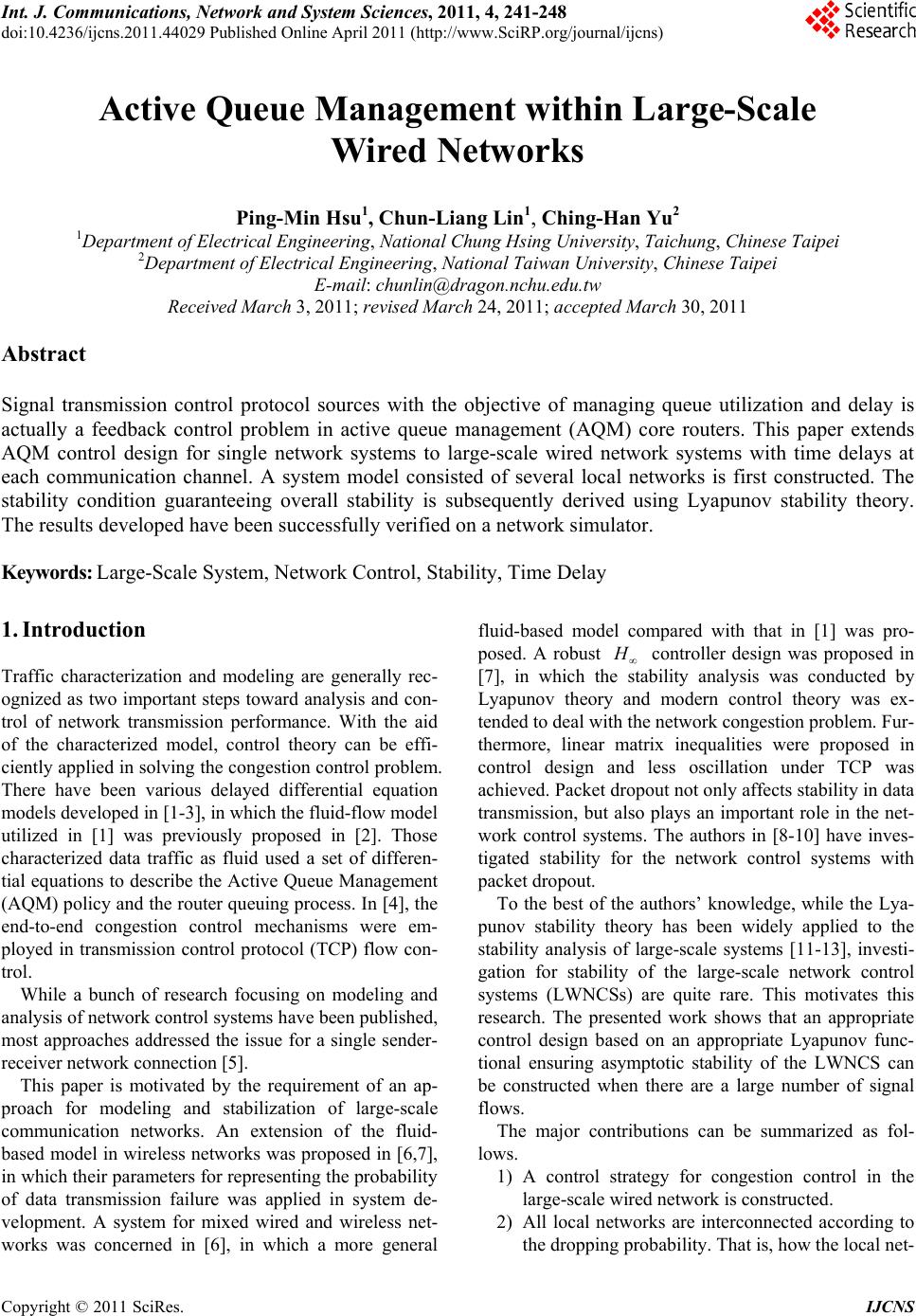
|