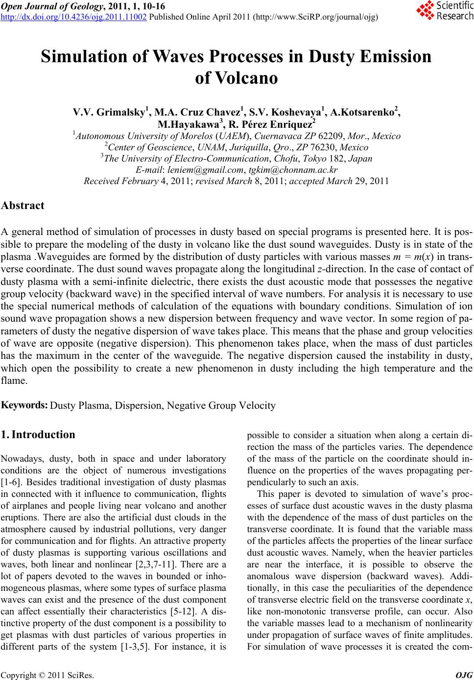Open Journal of Geology, 2011, 1, 10-16
http://dx.doi.org/10.4236/ojg.2011.11002 Published Online April 2011 (http://www.SciRP.org/journal/ojg)
Simulation of Waves Processes in Dusty Emission
of Volcano
V.V. Grimalsky1, M.A. Cruz Chavez1, S.V. Koshevaya1, A.Kotsarenko2,
M.Hayakawa3, R. Pérez Enriquez2
1Autonomous University of Morelos (UAEM), Cuernavaca ZP 62209, Mor., Mexico
2Center of Geoscience, UNAM, Juriquilla, Qro., ZP 76230, Mexico
3The University of Electro-Communication, Chofu, Tokyo 182, Japan
Received February 4, 2011; revised March 8, 2011; accepted March 29, 2011
Abstract
A general method of simulation of processes in dusty based on special programs is presented here. It is pos-
sible to prepare the modeling of the dusty in volcano like the dust sound waveguides. Dusty is in state of the
plasma .Waveguides are formed by the distribution of dusty particles with various masses m = m(x) in trans-
verse coordinate. The dust sound waves propagate along the longitudinal z-direction. In the case of contact of
dusty plasma with a semi-infinite dielectric, there exists the dust acoustic mode that possesses the negative
group velocity (backward wave) in the specified interval of wave numbers. For analysis it is necessary to use
the special numerical methods of calculation of the equations with boundary conditions. Simulation of ion
sound wave propagation shows a new dispersion between frequency and wave vector. In some region of pa-
rameters of dusty the negative dispersion of wave takes place. This means that the phase and group velocities
of wave are opposite (negative dispersion). This phenomenon takes place, when the mass of dust particles
has the maximum in the center of the waveguide. The negative dispersion caused the instability in dusty,
which open the possibility to create a new phenomenon in dusty including the high temperature and the
flame.
Keywords: Dusty Plasma, Dispersion, Negative Group Velocity
1. Introduction
Nowadays, dusty, both in space and under laboratory
conditions are the object of numerous investigations
[1-6]. Besides traditional investigation of dusty plasmas
in connected with it influence to communication, flights
of airplanes and people living near volcano and another
eruptions. There are also the artificial dust clouds in the
atmosphere caused by industrial pollutions, very danger
for communication and for flights. An attractive property
of dusty plasmas is supporting various oscillations and
waves, both linear and nonlinear [2,3,7-11]. There are a
lot of papers devoted to the waves in bounded or inho-
mogeneous plasmas, where some types of surface plasma
waves can exist and the presence of the dust component
can affect essentially their characteristics [5-12]. A dis-
tinctive property of the dust component is a possibility to
get plasmas with dust particles of various properties in
different parts of the system [1-3,5]. For instance, it is
possible to consider a situation when along a certain di-
rection the mass of the particles varies. The dependence
of the mass of the particle on the coordinate should in-
fluence on the properties of the waves propagating per-
pendicularly to such an axis.
This paper is devoted to simulation of wave’s proc-
esses of surface dust acoustic waves in the dusty plasma
with the dependence of the mass of dust particles on the
transverse coordinate. It is found that the variable mass
of the particles affects the properties of the linear surface
dust acoustic waves. Namely, when the heavier particles
are near the interface, it is possible to observe the
anomalous wave dispersion (backward waves). Addi-
tionally, in this case the peculiarities of the dependence
of transverse electric field on the transverse coordinate x,
like non-monotonic transverse profile, can occur. Also
the variable masses lead to a mechanism of nonlinearity
under propagation of surface waves of finite amplitudes.
For simulation of wave processes it is created the com-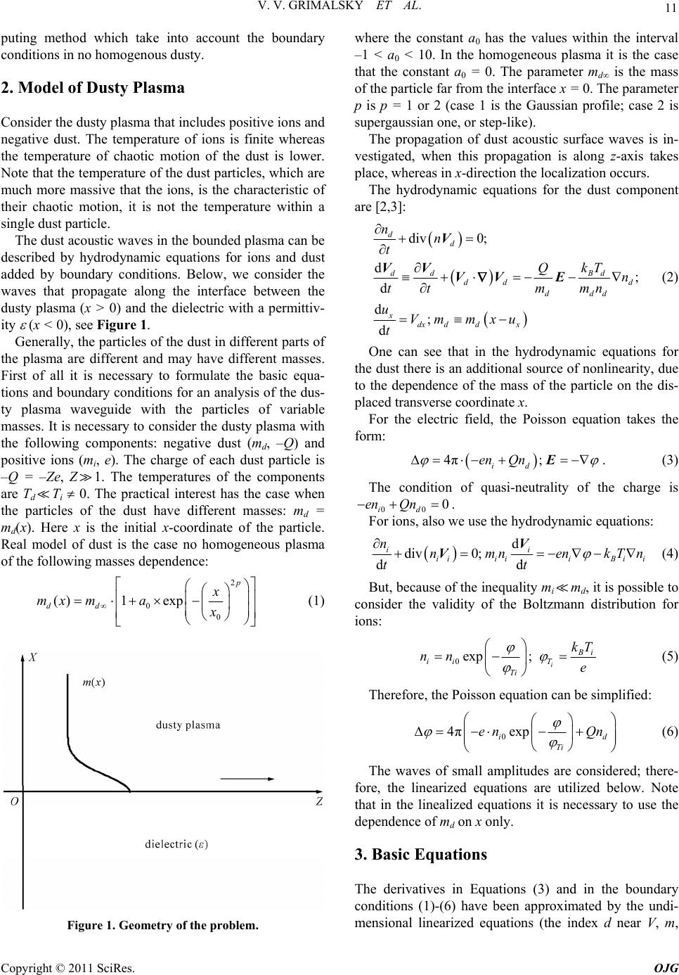

V. V. GRIMALSKY ET AL.
11
puting method which take into account the boundary
conditions in no homogenous dusty.
2. Model of Dusty Plasma
Consider the dusty plasma that includes positive ions and
negative dust. The temperature of ions is finite whereas
the temperature of chaotic motion of the dust is lower.
Note that the temperature of the dust particles, which are
much more massive that the ions, is the characteristic of
their chaotic motion, it is not the temperature within a
single dust particle.
The dust acoustic waves in the bounded plasma can be
described by hydrodynamic equations for ions and dust
added by boundary conditions. Below, we consider the
waves that propagate along the interface between the
dusty plasma (x > 0) and the dielectric with a permittiv-
ity
 (x < 0), see Figure 1.
Generally, the particles of the dust in different parts of
the plasma are different and may have different masses.
First of all it is necessary to formulate the basic equa-
tions and boundary conditions for an analysis of the dus-
ty plasma waveguide with the particles of variable
masses. It is necessary to consider the dusty plasma with
the following components: negative dust (md, –Q) and
positive ions (mi, e). The charge of each dust particle is
–Q = –Ze, Z1. The temperatures of the components
are TdTi  0. The practical interest has the case when
the particles of the dust have different masses: md =
md(x). Here x is the initial x-coordinate of the particle.
Real model of dust is the case no homogeneous plasma
of the following masses dependence:
2
0
0
()1 exp
p
dd
x
mx max




 
 






(1)
Figure 1. Geometry of the problem.
where the constant a0 has the values within the interval
–1 < a0 < 10. In the homogeneous plasma it is the case
that the constant a0 = 0. The parameter md is the mass
of the particle far from the interface x = 0. The parameter
p is p = 1 or 2 (case 1 is the Gaussian profile; case 2 is
supergaussian one, or step-like).
The propagation of dust acoustic surface waves is in-
vestigated, when this propagation is along z-axis takes
place, whereas in x-direction the localization occurs.
The hydrodynamic equations for the dust component
are [2,3]:



div 0;
d;
d
d;
d
d
d
dd Bd
dd d
ddd
x
dx ddx
nn
t
kT
Qn
tt mmn
uVm mxu
t




 


V
VV
VV E (2)
One can see that in the hydrodynamic equations for
the dust there is an additional source of nonlinearity, due
to the dependence of the mass of the particle on the dis-
placed transverse coordinate x.
For the electric field, the Poisson equation takes the
form:


4π;
id
en Qn



 E. (3)
The condition of quasi-neutrality of the charge is
00
0
id
en Qn

.
For ions, also we use the hydrodynamic equations:

d
div 0;
dd
ii
iiiiiBi i
nnmn enkTn
tt




V
V (4)
But, because of the inequality mimd, it is possible to
consider the validity of the Boltzmann distribution for
ions:
0exp; i
B
i
ii T
Ti
kT
nn e



 

 (5)
Therefore, the Poisson equation can be simplified:
0
4πexp
id
Ti
en Qn




 





(6)
The waves of small amplitudes are considered; there-
fore, the linearized equations are utilized below. Note
that in the linealized equations it is necessary to use the
dependence of md on x only.
3. Basic Equations
The derivatives in Equations (3) and in the boundary
conditions (1)-(6) have been approximated by the undi-
mensional linearized equations (the index d near V, m,

V. V. GRIMALSKY ET AL.
12
and n is omitted) can be represented as:
 
0
1;;
div 0;
Tnn
tmxmx
ñnnn
t







V
V
(7)
The following nondimensional variables have been
applied: x  x/rDi, z  z/rDi, V  V/Vn, t  t/tn,
 
 / 
Ti, m  m/m 
, ñ  ñ/nd0, T = Tde/TiQ  1. Here
the scale of the distance rDi = (kBTi/4e2ni0)1/2 is the De-
bye radius for ions, the characteristic velocity is Vn =
(QkBTi/em

)1/2, the time scale is tn = rDi/Vn. Therefore,
the undimensional mass of the dust particle is m(x) =
1 + a0exp(–(x/x0)2p). Note that the undimensional dust
temperature is a product of two small magnitudes Td/Ti <
1 and e/Q ~ 10–3 10–6, therefore, T < 10–3.
It is necessary to use the following algorithm of solu-
tion. First of all the traveling wave has view  , ñ 
exp(i(
 t – kz)).In this case, the set of equations (7) can
be reduced to the equations for the potential and for va-
riable part of the dust concentration:
 
 

22
2
2
2
2
d1d
dd
1d1 d0
dd
d10.
d
ñk ñ
xmx xmxT
k
Txmx xmxT
kn
x



 

 
 
 





 

(7)
It is necessary to add Equations (8) by the boundary
conditions. The continuity of the electric potential, the
x-component of the electric field (absence of the surface
charge at T  0), and zeroing vx-component of dust ve-
locity result in the boundary conditions at x = +0:
ddd
0; 0.
ddd
n
kT
xxx

  

Another boundary conditions are at x = Lxx0. In the
region xx0 the value of the nondimensional dust mass
is m = 1. In this region it is possible to reduce Equa-
tions (8):

22
2
2
2
2
2
d11
0;
d
d10
d
ñkn
TT x
kn
x




 


 


(10)
4. Simulation Method
The solution of (10) has the character to decreases at
xx0 like  , ñ ~ exp(-  x),  > 0. It takes the form:


 
112 2
111222
22
1,2 1,2
expexp ;
expexp ;
where 1
AxA x
ñ
A
xA x
k
 
 


 

(11)
In case of 
1,2 > 0 the solutions have following view:

2
2
22 222
1110kk
TT

 


 


.
Excluding the constants A1,2 from (11), one can get the
following boundary conditions at x = Lxx0:

21 121 2
12 12
12 21112 2
12 12
d0;
d
d0.
d
n
x
nn
x
  
 
  

 









(12)
It is necessary begin with simplified model where pa-
rameter T = 0. It is possible to obtain the single equation
for the potential only there:
 

2
dd 10.
dd
dd
xkx
xx






 (13)
A notation is used for the effective permittivity of the
plasma due to the dust component: 
d(x) = 1 – 1/(m(x)

2).
To get the waves localized in x-direction, it is necessary
to satisfy the condition () 0
dx

.
The boundary condition at x = +0 is:

d
00
d
dxk
x



, (14)
because the potential and x-component of the electric
induction are continuous there.
At x = Lxx0, it is possible to get the boundary con-
dition as:
22
2
d1 1
0,0,1 .
dd
d
k
x
 




 (15)
For the numerical solution of Equation (8) added by
boundary conditions (9) and (12), we have used the finite
differences [13]:








2
11
22
11
2
1/2 1/2
1
d1
|2;
d
d1d1 11;
dd
d1 ,where ,
d
j
j
N
xxjj j
jj jj
jj
xx
NNjj j
xx
xh
nnn nn
xmx xhmx mx
xxjh
xh

 
 












 
 (16)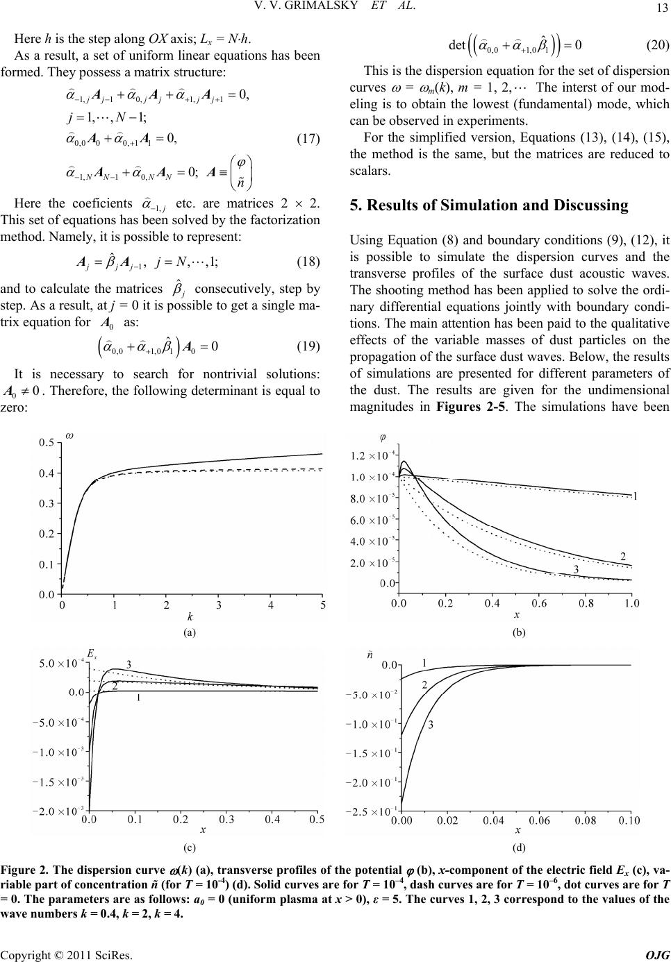

V. V. GRIMALSKY ET AL.
13
Here h is the step along OX axis; Lx = Nh.
As a result, a set of uniform linear equations has been
formed. They possess a matrix structure:
1,1 0,1,1
0,000, 11
1,1 0,
0,
1, ,1;
0,
0;
jjjj jj
NN NN
jN
n





 


 












AAA
AA
AAA
(17)
Here the coeficients 1,
j



etc. are matrices 2  2.
This set of equations has been solved by the factorization
method. Namely, it is possible to represent:
1
ˆ,,,1;
jjj
jN 

AA (18)
and to calculate the matrices ˆ
j

consecutively, step by
step. As a result, at j = 0 it is possible to get a single ma-
trix equation for 0 A as:

0,01,0 10
ˆ0




A (19)
It is necessary to search for nontrivial solutions:
00A. Therefore, the following determinant is equal to
zero:




0,01,0 1
ˆ
det 0 




 (20)
This is the dispersion equation for the set of dispersion
curves
 = 
m(k), m = 1, 2, The interst of our mod-
eling is to obtain the lowest (fundamental) mode, which
can be observed in experiments.
For the simplified version, Equations (13), (14), (15),
the method is the same, but the matrices are reduced to
scalars.
5. Results of Simulation and Discussing
Using Equation (8) and boundary conditions (9), (12), it
is possible to simulate the dispersion curves and the
transverse profiles of the surface dust acoustic waves.
The shooting method has been applied to solve the ordi-
nary differential equations jointly with boundary condi-
tions. The main attention has been paid to the qualitative
effects of the variable masses of dust particles on the
propagation of the surface dust waves. Below, the results
of simulations are presented for different parameters of
the dust. The results are given for the undimensional
magnitudes in Figures 2-5. The simulations have been
(a) (b)
(c) (d)
Figure 2. The dispersion curve  (k) (a), transverse profiles of the potential  (b), x-component of the electric field Ex (c), va-
riable part of concentration ñ (for T = 10-4) (d). Solid curves are for T = 10–4, dash curves are for T = 10–6, dot curves are for T
= 0. The parameters are as follows: a0 = 0 (uniform plasma at x > 0), ε = 5. The curves 1, 2, 3 correspond to the values of the
wave numbers k = 0.4, k = 2, k = 4.

V. V. GRIMALSKY ET AL.
14
(a) (b)
(c) (d)
Figure 3. The dispersion curve  (k) (a), transverse profiles of the potential  (b), x-component of the electric field Ex (c), va-
riable part of the dust concentration ñ (for T = 10–4) (d). Solid curves are for T = 10–4, dash curves are for T = 10–6, dot curves
are for T = 0. The parameters are as follows: a0 = 1 (heavier particles in the center of the waveguide), ε = 5, x0 = 0.25, p = 2. The
curves 1, 2, 3 correspond to the values of the wave numbers k = 0.4, k = 2, k = 4.
(a) (b)
Figure 4. The dispersion curves  (k) for dusty plasma waveguides with the heavier particles in the center of the waveguide.
Solid curves are for T = 10–4, dash curves are for T = 10–6, dot curves are for T = 0.The parameters are: (a) a0 = 1, ε = 5, x0 =
0.25, p = 1 (Gaussian profile); (b) a0 = 1, ε = 10, x0 = 0.25, p = 2 (step-like profile).

V. V. GRIMALSKY ET AL.
15
(a)
(a)
(c)
Figure 5. The dispersion curve  (k) (a), transverse profiles
of the potential
 (b), x-component of the electric field Ex
(c). Solid curves are for T = 10–4, dash curves are for T =
10–6, dot curves are for T = 0. The parameters are as follows:
a0 = –0.5 (lighter particles in the center of the waveguide),
x0 = 0.25, ε = 5, p = 2 (step-like profile of the mass). The
curves 1, 2, 3 correspond to the values of the wave numbers
k = 0.4, k = 2, k = 4.
realized for different dust temperatures T = 10–3 10–6,
and also for T = 0.
For uniform semi-infinite dusty plasma, the results of
simulations coincide with well-known data on surface
dust acoustic waves, see Figure 2. It is seen that the sur-
face plasma waves are preferably oscillations of the sur-
face charge. The localization thickness of the charge near
the surface is of about x ~ 0.010.02.
But the simulations of the dusty plasmas with variable
masses of the dust particles yield non-trivial results. One
can see that when the dust particles are heavier in the
center of the waveguide, it is possible to observe the
negative group velocity of surface waves at some inter-
vals of the wave numbers, see Figures 3, 4.
This result is tolerant to changes of parameters of the
dusty plasma waveguide, both for Gaussian and step-like
profiles of the masses of dust particles and also for dif-
ferent values of the dielectric permittivity of contacting
dielectrics. When the finite temperature of the dust is
taken into account, the negative dust velocity occurs at T 
10–4, whereas at higher temperatures this phenomenon
vanishes.
A possibility of opposite directions of phase and group
velocities of the surface plasma waves is important for
realization of wave instabilities, for instance, due to rota-
tion of dust particles [2]. Namely, as known from the
backward wave tube theory, the negative group velocity
can lead to positive distributed feedback within the sys-
tem [14,15]. The region of the wave numbers where the
group velocity of the wave is close to zero and changes
its sign can be also useful for observing nonlinear wave
phenomena, especially, envelope solitons or modulation
instability [14,16].
In the case of lighter particles in the center of the wa-
veguide, the group velocity is positive. But at some val-
ues of the wave numbers, the distribution of the trans-
verse Ex component of the electric field possesses
non-monotonic dependence on the transverse coordinate
x, see Figure 5.
This can be important for the dynamics of nonlinear
waves in this waveguide. The results on negative group
velocity have been confirmed by our more exact nu-
merical simulations of hydrodynamic equations, where
both the finite temperature of chaotic motion of dust par-
ticles and the finite mass of ions were taken into account.
6. Conclusion
To estimate the typical scales of the distance and time in
simulation, it is necessary to use the following parame-
ters: the temperature of the ions is Ti = 2000 K, the ion
concentration is ni0 = 103 cm–3, the radius of the dust
particle is rd = 10 µm, the mass of the dust particle far

V. V. GRIMALSKY ET AL.
16
from the boundary is m∞ = 2  10–8 g, the relation between
the charges of the dust particle and the ion is Q/e = 103.
In this case, the Debye radius for the ions (and the char-
acteristic spatial scale) is rDi = (kBTi/4e2ni0)1/2 10 cm;
the characteristic velocity is Vn = (kBTi/m∞ × Q/e)1/2  0.1
cm/s; the characteristic time is tn = rD/Vn  100 s  1.6
min.
When the dust particles are heavier in the center of the
waveguide, it is possible to observe the negative group
velocity of surface waves. So, this case is a good condi-
tion for obtain of the absolute instability of dust surface
plasma waves. This instability should be analyzed addi-
tionally. The estimated temporal and spatial scales have
demonstrated that it could be possible an appearance of
investigated phenomena under natural hazards, like vol-
cano eruptions.
7. Acknowledgements
Authors are grateful to CONACyT (Mexico) for a partial
financial support of our work.
8. References
[1] V., Fortov, A. Ivlev, S. Khrapak, A. Khrapak and G.
Morfill G.E., “Complex (dusty) plasmas: Current status,
open issues, perspectives”, Physics Reports, Vol. 421, No
1-2, 2005, PP. 1-103.
[2] Shukla, P., Mamun, A. (2002) Introduction to Dusty
Plasma Physics. Bristol, Institute of Physics Publ.
[3] Verheest F., (2000) Waves in Dusty Space Plasmas. Dor-
drecht, Kluwer Publ.
[4] P. Shukla and A. Mamun, “Solitons, shocks and vortices
in dusty plasmas”, New Journal of Physics, Vol. 5, No 1,
2003, PP.17.1-17.37.
[5] S. Popel, S. Kopnin, I. Kosarev, M. Yu, “Solitons in
Earth’s dusty mesosphere”, Advances in Space Research,
Vol. 37, No 2, 2006, PP. 414-419.
[6] P. Shukla, “A survey of dusty plasma physics”, Physics
of Plasmas, Vol. 8, No 5, 2001, PP. 1791-1803.
[7] K. Ostriko, M. Yu and L. Stenflo, “Surface waves in
strongly irradiated dusty plasmas”, Physical Review E,
Vol. 61, No 1, 2000, PP. 782-787.
[8] B. Klumov, G. Morfill, S. Popel, “Formation of Struc-
tures in a Dusty Ionosphere”, Journal of Experimental
and Theoretical Physics, Vol. 100, No 1, 2005, PP. 152-
164.
[9] Kopnin S., Popel S. (2005) Dust Acoustic Mode Mani-
festations in Earth’s Dusty Ionosphere, AIP Conference
Proceedings, Vol. 799, PP. 161-164.
[10] S. Popel, M. Yu, V. Tsytovich, “Shock waves in plasmas
containing variable charge impurities”, Physics of Plas-
mas, Vol. 3, No 12, 1996, PP. 4313-4315.
[11] S. Popel, A. Golub’, T. Losseva, R. Bingham and S.
Benkadda, “Evolution of perturbation in charge-varying
dusty plasmas”, Physics of Plasmas, Vol. 8, No 5, 2001,
PP. 1497-1504.
[12] V, Grimalsk, S. Koshevaya, R. Perez-Enriquez, A. Kot-
sarenko, “Interaction of linear and nonlinear ion-sound
waves with inclusions of dusty plasma”, Physica Scripta,
Vol. 74, No 3, 2006, PP. 317-324.
[13] Samarskii, A., (2001) The Theory of Difference Schemes.
N.Y., Marcel Dekker.
[14] Infeld, E., and Rowlands G. (2000) Nonlinear Waves,
Solitons and Chaos. Cambridge University Press, Cam-
bridge.
[15] Lifshitz, E., Pitaevskii, L. (1981) Physical Kinetics.
London, Pergamon.
[16] Ostrovsky, L., Potapov, A., (2002) Modulated Waves:
Theory and Applications. N.Y., The Johns Hopkins Uni-
versity Press.