Journal of Applied Mathematics and Physics, 2014, 2, 365-383
Published Online May 2014 in SciRes. http://www.scirp.org/journal/jamp
http://dx.doi.org/10.4236/jamp.2014.26044
How to cite this paper: Svensson, U. and Ferry, M. (2014) DarcyTools: A Computer Code for Hydrogeological Analysis of
Nuclear Waste Repositories in Fractured Rock. Journal of Applied Mathematics and Physics, 2, 365-383.
http://dx.doi.org/10.4236/jamp.2014.26044
DarcyTools: A Computer Code for
Hydrogeological Analysis of Nuclear Waste
Repositories in Fractured Rock
Urban Svensson1, Michel Ferry2
1Comput er-aided Fluid Engineering AB, Frankes väg 3, 371 65 Lyckeby, Sweden
2MFRDC, 6 rue de la Perche, 44700 Orvault, France
Received January 2014
Abstract
A computer code for simulation of groundwater flow and transport is described. Both porous and
fractured media are handled by the code. The main intended application is the analysis of a deep
repository for nuclear waste and for this reason flow and transport in a sparsely fractured rock is
in focus. The mathematical and numerical models are described in some detail. In short, one may
say that the code is based on the traditional conservation and state laws, but also embodies a
number of submodels (subgrid processes, permafrost, etc). An unstructured Cartesian grid and a
finite volume approach are the key elements in the discretization of the basic equations. A multi-
grid solver is part of the code as well as a parallelization option based on the SPMD (Single-Pro-
gram Multiple-Data) method. The main application areas are summarized and an application to a
deep repository is discussed in some more detail.
Keywords
Fractured R ock, Inflow Prediction, Deep Repository
1. Introduction
1.1. Background
DarcyTools is a computer code for simulation of flow and transport in porous and/or fractured media. The frac-
tured media in mind is a fractured rock and the porous media is the soil cover on the top of the rock; it is hence
groundwater flow, which is the class of flows in mind. The code is intended to be applicable to a wide range of
groundwater flows, but the analysis of a repository for nuclear waste is the main intended application. For the
present purposes, the repository can be defined as a set of tunnels and holes for deposition of canisters. It is fur-
ther expected that the repository will be placed at a depth of about 500 metre, in a sparsely fractured rock.
Flow and transport in a sparsely fractured rock is due to a system of fractures and faults, spanning scales from
mm to km. A groundwater model should hence represent this network of fractures and then simulate the flow
and transport in the network.

U. Svensson, M. Ferry
366
Two basic approaches in groundwater modelling can be identified; in one, grid cell conductivities are defined
(sometimes called the continuum porous-medium (CPM) approach, e.g. [1]), while in the other, the flow through
the network is calculated directly (discrete fracture network (DFN) approach). Both approaches have their merits
and drawbacks, though these will not be discussed in this paper (for discussions, see e.g. [2] [3],). DarcyTools is
based on a method that combines the approaches, meaning that a fracture network is first generated and then the
network is represented as grid cell conductivities. The resulting property fields are expected to have some desir-
able features, such as realistic correlation and anisotropy structure, provided the network is properly represented
in the grid.
DarcyTools uses an unstructured Cartesian grid, that allows for local refinements around tunnels, boreholes,
fracture zones, etc. After the equations have been discretized, using a finite volume approach, the resulting sys-
tem of equations is solved by a multigrid solver. For a detailed description of the code and its use, the reader is
referred to three reports that give a full account of the code ([4]-[6]).
A number of well-established codes for repository analysis are available: TOUGH2 [7], MODFLOW [8],
PFLOTRAN [9], Connect Flow [3] and FRACMAN [10] to mention a few. In order to relate DarcyTools to
these codes some strong points and limitations of DarcyTools are listed.
Strong points:
• A fracture network, built on both deterministic and random fractures, is easily generated or imported from
another fracture generator. Sub grid fractures are considered by a sub grid model.
• An unstructured grid resolves objects (repository, lakes, fracture zones, etc) read in as CAD files. Computa-
tional cells can be removed or refined according to various criteria.
• Efficient numerical solutions; multigrid techniques, parallelization, etc.
Limitations:
• Chemical reactions and multiphase flow are not simulated by DarcyTools.
• Thermo-hydro mechanical effects [11] are not handled in the present version of DarcyTools.
1.2. Objective
The main objective is to describe the computer code Dar c yToo ls. The scope, features, basic equations, numeri-
cal methods and an application to a deep repository case will be briefly described.
2. Scope
2.1. Introduction
Simulations for the analysis of a nuclear waste repository are, as stated, the main intended application. This,
however consists of a broad range of simulations, both with respect to space and time scales. Simulations of the
flow below inland ice sheets (relevant in long term scenario studies of a repository) with very large space and
time scales may be considered, contrasted with transport at the interface between a deposition hole and the rock
(flow and diffusion on the mm scale). In this section, the scope will be illustrated by a discussion of the proc-
esses on scales ranging from the 10 km scale down to the mm scale.
2.2. The 10 km Scale View
The regional groundwater flow in unconfined aquifers introduces the concepts of recharge and discharge areas,
see Fig ure 1. Recharge areas, i.e. where a net inflow is found, are usually found in topographically high places
while the discharge areas are located in topographic lows. A discharge area may take the form of a stream, river
or a lake.
The general flow pattern is thus from high to low areas; a system of local flow cells is formed and the
groundwater table follows the surface topography. However, this is an idealized picture based on the assump-
tions of a steady and constant density flow in a homogeneous aquifer. These assumptions are seldom fulfilled
and care should hence be taken when interpreting field data. In particular, most natural aquifers are anisotropic
and heterogeneous.
2.3. The km Scale View
A km scale view is provided in Figure 1. Let us assume that it is of interest to determine the origin of water

U. Svensson, M. Ferry
367
Figure 1. Situations considered. The 10 km scale view (top)
and the km scale view.
leaking into a tunnel. Two main sources of water are precipitation and sea water (excluding brine water from
below). To track the precipitation water it is needed to follow a water parcel through the unsaturated zone,
through the saturated soil cover and finally its way through the fracture network. It is essential to determine the
position of the groundwater table, as it determines the pressure gradients in the porous medium and may influ-
ence the conditions deep in the rock. The other source, the sea water, introduces density effects, as the seawater
has higher density than fresh water. The heavier saltwater penetrates the coastal zone and modifies the pressure
distribution (the Ghübern Herzberg relation). Due to this effect the inflow into the tunnel may be dominated by
sea water or precipitation water depending on the actual conditions (density difference, tunnel position, etc).
2.4. The m Scale View
The main novel features of DarcyTools are concerned with the fracture network and focus will therefore be on
the description of fractures (giving the porous media less attention). In Fig ure 2 part of a fracture network is
shown. Different parts of the network have been marked with letters; these parts will now be described:
A: Represents a fracture zone. The fracture zone is assumed to be composed of a number of smaller fractures
through which the flow takes place. However, most of the small fractures do not contribute to the flow but are
important nonetheless for transport and dispersion of a tracer. Fracture zones are often the main flow conductors
due to their high transmissivity and size (length scale >100 metres). The typical thickness is >1 metre.
B: Some fractures are best characterized as “a single opening”. The typical thickness, or the aperture, is on the
order of 10−3 metres. The fractures marked with B in Fig ure 2 have a through-fl ow and may thus contribute to
the total flow rate. If the transport time through the B fractures is different from the transport time in the fracture
zone, a dispersion effect will also result from the parallel flow path.
C: Isolated fractures, or groups of isolated fractures, cannot contribute to the flow, transport or dispersion, as
flow in the matrix is normally neglected. In the numerical model these are removed prior to grid data generation.

U. Svensson, M. Ferry
368
Figure 2. Situ ations considered. The m scale view (top) and
the mm scale view.
D: Some fractures, or fracture zones, may form “dead end systems”. The exchange with fractures with sig-
nificant flows is then by molecular diffusion. When solute transport or storage of water over long time periods,
say longer than 100 years, is studied it is essential to represent the dead-end systems correctly.
E, F: There is always a lower limit on the fracture size that can be correctly represented in a numerical simu-
lation. In the present formulation, it will be assumed that fractures below a certain size do not contribute signifi-
cantly to the total flow. However, for transport and dispersion it is probably necessary to consider all scales, as a
large fraction of the pore volume is expected to be due to the small scale features of the fracture network.
2.5. The mm Scale View
It was mentioned above that the opening, or aperture, of a fracture is typically on the order of 1 mm or smaller.
However, the aperture does not have a constant value, as is illustrated in Figure 2. On this scale, it is useful to
introduce the notions of the mobile zone for the volume that has flowing water and the immobile zone, which
represents all volumes with stagnant water. In Figure 2, the stagnant pools, the crossing fractures and the matrix
may all contain stagnant water. The fracture may also contain geological material of various kinds, so called
gouge material.
It is essential to consider the geometrical complexity of a fracture opening when describing small scale dis-
persion processes. The exchange between the mobile and immobile zones is often assumed to be due to molecu-
lar diffusion only.
3. Main Features
The main features of DarcyTools are summarized in Table 1. In short, one may say that a fracture network is
represented on an unstructured Cartesian grid and the resulting finite volume equations are solved by a multigrid
solver. An elaboration of some of the features listed in Table 1 follows below:
• Fracture network. Deterministic fractures and fracture zones are assumed to be known with respect to posi-
tion and extent. Other properties, such as transmissivity, may also have been evaluated from field tests.
Random fracture sets are generated with a power law for size distribution and a Fisher distribution for or ie nt-

U. Svensson, M. Ferry
369
Table 1. Main features.
Feature Description
Fracture network Network with deterministic and random fractures. Fisher
distribution for orientation. Heterogeneous fractures.
Matrix exchange A multi-rate, or single rate, diffusion concept. Handles both particles
and advection/diffusion equations.
Free groundwater surface An algorithm that focuses on the position of the groundwater table.
Particle tracking Two options, traditional flow following and a cell-jump method.
Tunnels and boreholes Introduced as CAD-objects. Routines for setting pressure and grouting conditions.
Water type analysis A series of advection/diffusion equations are solved to track
waters of different origin (in space and time).
Gravitational effects, buoyancy Full coupling through the density laws with salinity and temperature fields.
Basic equations Darcy’s law. Conservation equations. State laws for properties.
Grid system Unstructured Cartesian grid.
Representation of fractures on the grid Cell properties calculated according to the intersecting volumes between fractures and cells.
Discretization method Finite volumes. Hybrid schemes.
Solver, parallelization Multigrid solver. SPMD (Single Program Multiple Data) parallelization.
tation. Normally a Poisson distribution is used for spatial positions. Random fractures, or groups of fractures,
may be removed if isolated. A limited number of deterministic fractures can be given heterogeneous proper-
ties (in order to achieve channelling effects for flow).
• Matrix exchange. Fractures that cannot be explicitly represented in the computational grid are handled by a
subgrid model. This model is based on the multi-rate diffusion model [12] and an assumption of a power law
for fracture size distribution. The subgrid model is implemented both for advection/diffusion equations, for
example used for salinity, and for a particle tracking routine. A single-rate option for simulating a matrix
with uniform properties is also implemented.
• Free groundwater surface. The free surface algorithm focuses on the position of the groundwater table. The
position is determined by the local mass balance, but does not consider the properties of the unsaturated
zone.
• Tunnels and boreholes. The grid generator reads the CAD files for these objects and refines the grid locally
around the objects according to various criteria. Grouting around tunnels can be simulated by putting condi-
tions on the hydraulic conductivity in layers around the tunnel. Various boundary conditions (fixed inflow,
fixed pressure, etc) can be associated with the objects.
• Representation of fractures on the grid. The basic technique is described in detail in [13] and [14]. In these
papers it is shown that the method is accurate and effective.
4. Mathematical Formulation
4.1. Introduction
The mathematical formulation is straightforward as the conservation and state laws are formulated in a fairly
standard way.
4.2. Conservation Laws
Conservation of mass:
( )( )( )
uv wQ
txy z
ρθ ρρρ ∂∂∂ ∂
+++ =
∂∂∂ ∂
(1)
where
ρ
is fluid density θ, porosity, u, v and w Darcy velocities and Q a source/sink term. The coordinate

U. Svensson, M. Ferry
370
system is denoted x, y, z (space) and t (time).
Mass fraction transport equation:
x yzC
CC CC
uCDvCDwCD QCQ
txxyyz z
ρθ ρργρ ργρργ  ∂∂∂∂∂∂ ∂
 
+−+−+ −=+

 
∂∂∂∂∂∂ ∂
 

(2)
where C is transported mass fraction, Dx, Dy and Dz the normal terms of the diffusion-dispersion tensor and Qc a
source/sink term, that represents the exchange with immobile zones. Note that the diffusion coefficients are the
effective coefficients that include the porosity, see further explanation of the diffusion term in connection with
Equation (11) below.
Conservation of heat:
()
(1 )
p
pxpypzpT
c cTTT T
ucTvcTwcTQcT Q
txxyyz z
ρθ θρλρλρ λ
∂ +−
∂∂∂∂∂ ∂
 
+−+ −+−=+

 
∂∂∂∂∂∂ ∂
 

(3)
whe r e
x
λ
,
y
λ
and
z
λ
are the normal terms of the equivalent (i.e. rock with fluid) thermal conductivity tensor, c
is the rock thermal capacity and cp the specific heat of the fluid and
T
Q
a source/sink term. We are hence only
solving for one temperature, assuming thermal equilibrium between the rock and the water. Note that we have
chosen to use c (Joul e/ m3 ºC) for the rock thermal capacity and
p
c
(Joul e/ kg ˚C) for the specific heat of the fluid.
The reason for this inconsistency is that this formulation does not require the rock density as an input variable.
The mass conservation equation is turned into a pressure equation under the well-known Darcy’s law:
0
()
x
y
z
z
KP
ugx
KP
vgy
KP
wK
gz
ρ
ρ
ρ ρρ
∂
= −∂
∂
= −∂
∂
=− −−
∂
(4)
where Kx, Ky and Kz are the local hydraulic conductivities in x, y and z direction, g the gravity acceleration, ρ0 a
reference fluid density and P the dynamic fluid pressure relative to the reference hydrostatic pressure
0
P pgz ρ = +
(5)
where p is the total pressure. The hydraulic conductivity, K, is related to the permeability, k, by the relation:
gk
K
ρ
µ
=
(6)
where μ is the dynamic viscosity.
4.3. State Laws
The fluid properties like the dynamic viscosity,
µ
, the density,
ρ
, and the specific heat,
p
c
, are given by
state laws:
( )( )
2
01 2
1
n
aTT aTT
µ
µµ
µµ

=+ −+−


(7)
() ()
2
2
012 12
1S STTTT
ρρ
ρρα αββ

=++−−−−


(8)
( )
2
0 12
1
pp
ccbSbS= ++
(9)
while the porosity
θ
and the compaction,
γ
, of the matrix are given the following dependencies:
0
θ θγ =
(10)
00
1 ()()PP g γ σθρ =+−
(11)

U. Svensson, M. Ferry
371
In the above formulas S represents the salinity (salt mass fraction),
0
θ
a reference porosity field given for a
reference pressure field P0 and
σ
the specific storativity field.
n
µ
,
i
a
,
i
b
,
i
α
,
i
β
,
0
µ
,
0
ρ
,
0p
c
,
T
µ
and
T
ρ
are constants. Equations (7) to (9) thus provide linear and quadratic dependencies of salinity and temperature. It is
the user’s task to find the best coefficients for a given problem.
In the advection/diffusion Equation (2), it is common to write the diffusion coefficient as
mol
D θ
, where
mol
D
is the molecular diffusion coefficient. In DarcyTools we choose to write the term as
0mol mol
D DD θ θγγ = =
,
where D is now the effective diffusion coefficient.
4.4. Additional Models
DarcyTools embodies a number of additional special purpose models. The most important of these are:
• Subgrid model. When the transport of a substance (salt, radionuclide, etc.) is to be analyzed, it is necessary to
consider processes on the mm scale, see Figure 2. A number of processes, on a range of time and space scales,
contribute to the dispersion of a substance as it travels with the flow. The processes on the mm scale are often
very significant and DarcyTools includes a sub grid model [12], to deal with these processes.
• Permafrost model. DarcyTools contains a model to simulate the permafrost freezing and thawing process. To
take into account the phase change of water when the temperature goes below the melting-point, the source
terms of Equations (1), (2) and (3) are modified. Properties such as permeability or thermal conductivity are
also highly dependent on the ice content.
• Grouting model. As mentioned in Section 3, the hydraulic conductivity in the near field of a tunnel can be
modified, in order to simulate the effect of grouting.
5. Numerical Methods
5.1. Introduction
The conservation laws are represented on a computational grid using the finite volume method. The finite vol-
ume method integrates equations over the faces of a finite number of control volumes by converting volume in-
tegrals into surface integrals using the Ostrograd sky and the mean value theorems:
1
()
nbfaces
ii i
VV
i
divFdVFndAA Fn
∂=
= ⋅=⋅
∑
∫∫
 

(12)
where, Ai and ni are respectively the area and the outside-normal of the cell face named i and where the flux value
Fi is evaluated at face centre.
5.2. Discretization in Space
Among the common grid arrangements, DarcyTools uses the “cell-centred” arrangement [15] in which the
pressure and the scalar variables (mass fractions) are located at centre of grid cells, see Figure 3 and Figure 4. The
Figure 3. Unstructured Cartesian control vol-
umes, faces and normals.

U. Svensson, M. Ferry
372
Figure 4. Cell-centred arrangement labelling.
main advantage of this formulation is the fact that control volumes coincide with grid cells and that cell vertexes
are directly defined by grid nodes. The main drawback is the fact that, for non-uniform meshes, the faces of
control volumes may not be located mid-way between variable locations or may not be orthogonal to the line
joining cell centers. More sophisticated interpolations are therefore necessary to get a second order discretization
of convective and diffusive fluxes.
For stability reasons the discretization in space of Equations (1), (2) and (3) involves both convective and
diffusive fluxes according to the Hybrid Differencing Scheme [16]. This scheme (13) is based on a combination of
central and upwind differencing schemes depending on the value of the local Peclet number. For Peclet numbers
smaller than two the scheme is second order while for higher Peclet numbers it is only accurate to first order but
accounts for transportiveness [17]
*() i PE
i
F c daca
x
φ
φ φφ
∂

= −=+−

∂

(13)
2
max0,,hc d ac
hh
+
+−

+
=
+

(14)
( )
*() PP P
PEPE nngrad φφ φ =+−
 
(15)
where h+ and h− represent respectively the size of cell E and cell P and where the cell centred gradient is given by
the Gauss theorem as:
1
1nbfaces
i ii
i
gradA n
V
φφ
=
=
∑
 
(16)
where V represents the volume of the cell and
i
φ
the face value of the quantity under consideration.
* iP E
hh
hh hh
φφ φ
+−
+− +−
= +
++
(17)
Since in Equation (16) the face values (17) are linked to the gradient through (15), the gradient value is obtained
after some iterations of a fix point algorithm. Three iterations produce a sufficient accuracy for most uses.
5.3. Time Discretization
To ensure the precision of time dependent simulations, when users specify transient boundary conditions and time
variations of time steps, Darc yTools discretizes the time derivative term of Equations (1), (2) and (3) as a fully
implicit second order backward finite difference:

U. Svensson, M. Ferry
373
(18)
where ∆t1 and ∆t2 represent respectively the time steps tn − tn−1 and tn-1 − tn−2. However, a first-order backward
implicit Euler scheme, less demanding in memory, is also possible for simply relaxing non-linear steady flow
simula t io ns:
1
1
nn
nnn
t tt
φφ
φ
−
−
−
∂=
∂−
(19)
5.4. Cartesian Grids
With structured grids, local refinements may drastically increase the total number of cells by propagating cell
size reductions up to boundaries, see Figure 5. To avoid this generation of useless cells in regions of low inter-
est, DarcyTools uses adaptive Cartesian grids [18]. Starting with a single cell that covers the entire domain, the
grid generator successively splits cells requiring refinement in two half children cells and repeats this procedure
for each direction until the cell size, or the total number of cells, reaches threshold values.
These threshold values as well as cell removal criteria are user defined during the initial grid construction but
also during any grid update according to rock properties. Zones with different cell sizes, or cell removal criteria,
may be defined from predefined objects such as lines, planes, parallelepipeds, cylinders or spheres, but mainly
from real triangulated shapes stored from CAD software using the STL (Stereo Lithography) file format.
Though cell information could be stored in an octree data structure, DarcyTools implements a fully unstruc-
tured data structure where cell locations and sizes are stored in a compact structure using only fifteen bytes per
cell.
5.5. Solve r
DarcyTools uses a GMRES Krylov subspace solver [19] in association with a multigrid preconditioner [20] to
achieve a fast and robust convergence of the algebraic sets of equations resulting from successive discretizations.
To simultaneously adapt its coarse grid operators to the unstructured Cartesian grid and to the rock properties,
the multigrid preconditioner in use is based on an algebraic multigrid method [21] which uses only the informa-
tion available in the linear system of equations.
The multigrid method improves the reduction of long wave length error components, which is important for
solving the mass conservation equation with iterative methods. The GMRES method ensures the robustness of the
solver when sharp variations of physical properties in the fractured rock ill-condition the algebraic sets of equa-
tions for the Incomplete Lower-Upper factorization (ILU0) smoother.
When the buoyancy term of Equation (4) slows down the convergence, because of the non-linear coupling
between the mass conservation equation and the salt transport equation, DarcyTools uses one of the capabilities
of its multigrid preconditioner [22] which consists in simultaneously iterating both equations in a strongly
coupled manner in order to accelerate the global convergence.
Figure 5. Structured vs unstructured grids.
2
212
1
1
21
21
211
21
)()(
2
−− ∆+∆∆
∆
+
∆∆
∆+∆
−
∆+∆∆
∆+∆
=
∂
∂
nnn
nttt
t
tt
tt
ttt
tt
t
φφφ
φ

U. Svensson, M. Ferry
374
5.6. Paralleli zat i on
The parallelization techniques employed in DarcyTools rely on a Single-Program Multiple-Data (SPMD) ap-
proach which consists in first partitioning the grid and then in executing the same piece of code repeatedly on each
block.
By default, DarcyTools automatically partitions the domain using a Hilbert space-filling curves technique,
taking advantage of the Cartesian structure of the grid [23] and [24]. Given a list of cells in the original domain, a
space-filling curve is built that passes through each cell once, see Figure 6. The map is constructed so that cells
that are close in 3D space remain close when mapped. Thus, the curve preserves locality. Once the curve is con-
structed, the decomposition of the domain is performed by dividing it into N subintervals, where N is the number
of processors to be used. For load balancing the length of any subinterval can be specified in term of percentage of
the total length. When load balance is crucial, users may specify their own partition.
To avoid scalability limitations due to memory bandwidth, and to enable runs on distributed memory clusters,
DarcyTools implements the Message-P as sin g-Interface (MPI) technique for communication between the blocks
of the domain. This choice does not restrict the applicability of DarcyTools to clusters since the same MPI tech-
nique equally applies on multi-core shared memory computers.
6. Application Areas
Even if a wide range of groundwater flow problems can be simulated with DarcyTools, most applications have
so far been related to the analysis of a nuclear waste repository. The Forsmark site (located around 120 km north
of Stockholm, Sweden) is of particular significance as the Swedish Nuclear Fuel and Waste Management Com-
pany (SKB) has submitted a license application for the construction of a final repository at this site. An intro-
duction to the Forsmark site, and the modelling tasks carried out, is given by [25]. For the present objectives we
show a map over the area, see Fig ure 7, and note that it is a coastal site with a number of small shallow lakes.
The application areas are summarized in Table 2 and an elaboration is given by the following points:
• Site investigations. At Forsmark, the water in the bedrock is saline with a salinity that increases with depth.
The resulting density field will influence the undisturbed flow pattern and it is hence of interest to simulate
and understand the present day salinity distribution. Simulations covering a period of about 10,000 years
(since the last glaciation) have been carried out considering the variation in water level and salinity of the
Baltic Sea during the period.
• Open repository. The open phase of a repository is expected to be around 50 years and during this time in-
terval different parts of the repository will be opened and closed successively. It is of interest to know the in-
flow distribution, in space and time, during this phase as the inflow is related to effects like drawdowns of
the groundwater table and upconing of salt water from below the repository. One way to control the inflow
rate is by grouting, a process that also needs to be simulated in order to estimate the reduction of the inflow.
The open phase of the Forsmark repository will be discussed in more detail in the next section.
Figure 6. Example of Paneo-Hilbert space-fill-
ing curve partitioning.

U. Svensson, M. Ferry
375
Figure 7. The red polygon shows the size and location of the candidate area for site investigations at Forsmark.
The green rectangle indicates the size and location of the regional model area used in the analysis of the site.

U. Svensson, M. Ferry
376
Table 2. Key application areas.
Application Description
Site Investigation Development of salinity field since last glaciation. Natural flow system.
Water type evolution. Super regional models. Borehole analysis.
Open repository Inflow distribution in space and time. Draw downs. Resaturation of backfill. Grouting.
Permafrost and Glaciation Long term scenarios. Ice sheets.
Surface hydrology Surface waters and their interaction with the groundwater system.
Transport in lakes, streams and near ground.
Transport and retention Transport of radionuclides from a deposition hole to ground surface. Reactive transport.
• Transport and retention. After closure of the repository there will be a stage during which the tunnel backfill
and the bentonite clay enclosing the canisters are saturated. After this stage a flow pattern that is close to the
undisturbed situation can be expected. The whole transport path, from the canister, through the fracture net-
work and through the lakes and streams then needs to be analyzed. Close to the canisters matrix diffusion
may be the dominating mode of transport.
• Surface hydrology. In the performance and safety assessment of a repository, it is of interest to include the
surface water system (lakes and streams) for at least two reasons: 1) During the operational phase one can
expect a drawdown of the groundwater table, due to the inflow to the open repository. This drawdown needs
to be estimated due to its environmental impact. 2) Lakes and streams provide a link in the transport chain
from a deposition hole to the sea. All parts of the possible transport paths are essential to understand.
• Permafrost and Glaciation. The objective of these studies is to provide bounding hydrogeological estimates
at different stages during glaciation and deglaciation of a glacial cycle [26].
7. The Open Phase of the Forsmark Repository
7.1. Introduction
The main objective of the modelling of the open phase is to evaluate the hydrogeological effects caused by an
open repository. In particular, the following is studied:
• the magnitude and spatial distribution of the inflow to the open repository,
• the magnitude and spatial distribution of the drawdown of the groundwater table,
• the chemical composition (i.e. salinity) and spatial distribution of the groundwater in proximity of the open
repository,
• the role of grouting for the inflow, drawdown and upconing phenomena, and
• the saturation period after the open repository has been closed (backfilled).
The mathematical modelling of the repository considers three operation stages, A-C (see Figure 8), which
were run in sequence, where the first stage, stage A, lasted for 15 years, stage B lasted for 15 years and stage C
lasted for 20 years. Hence, the total operation time was 50 years. The role of grouting was looked at by model-
ling three levels of grouting efficiency, I-III, see Table 3. A full account of this work can be found in [27]; here
we will focus on the set-up of the computational grid and some results concerning inflow to the repository.
7.2. Set-Ups
The computational grid was refined in the vicinity of the repository in order to resolve the repository layout and
to study the effects of grouting. The largest cell size away from the repository was 128 metres (Figure s 9-11)
and in the proximity of the repository the cell size was 4 metres. This high resolution was needed to resolve the
deposition tunnels, which have a height of 4.8 metres and width of 4.2 metres. A vertical cross-section through
the repository is shown in Figure 12; the vertical resolution of the cells close to the top boundary was 2 metres.
In total about 1.4 million cells were used to model the problem as outlined.
The geometry and hydraulic properties of discrete geological features in the bedrock such as deformation
zones, sheet joints and fracture network realizations were imported from the work by [28]. The vertical perme-
ability field around the repository, as represented on the grid, is shown in Figure 13.

U. Svensson, M. Ferry
377
Figure 8. Definition of different parts of the studied repository layout
at Forsmark. The mathematical modelling considers three operation
stages, A-C, and three possible grouting levels for each stage. The
three stages are indicated by green, turquoise and pink colours. DA =
deposition area, MT = transportation and main tunnel, VS = ventila-
tion shaft, CA = central area. The deposition tunnels are shown as
branches to the main tunnels and the canister holes (almost invisible)
are drilled from the bottom of the deposition tunnels.
Figure 9. Plan view of the model area and the computa-
tional grid at −465 m elevation. The size of the largest grid
cells is 128 m.
Table 3. Definition of the studied levels of grouting efficiency.
Level Definition
I The hydraulic conductivity of all cells in contact with the repository has a maximum value of 1 × 10−7 m/s.
II The hydraulic conductivity of all cells in contact with the repository has a maximum value of 1 × 10−8 m/s.
III
The hydraulic conductivity of all cells in contact with the repository has a maximum value of
1 × 10−9 m/s except where the modelled ungrouted hydraulic conductivity is 10−6 m/s or greater.
At these positions the hydraulic conductivity has a maximum value of 1 × 10−8 m/s.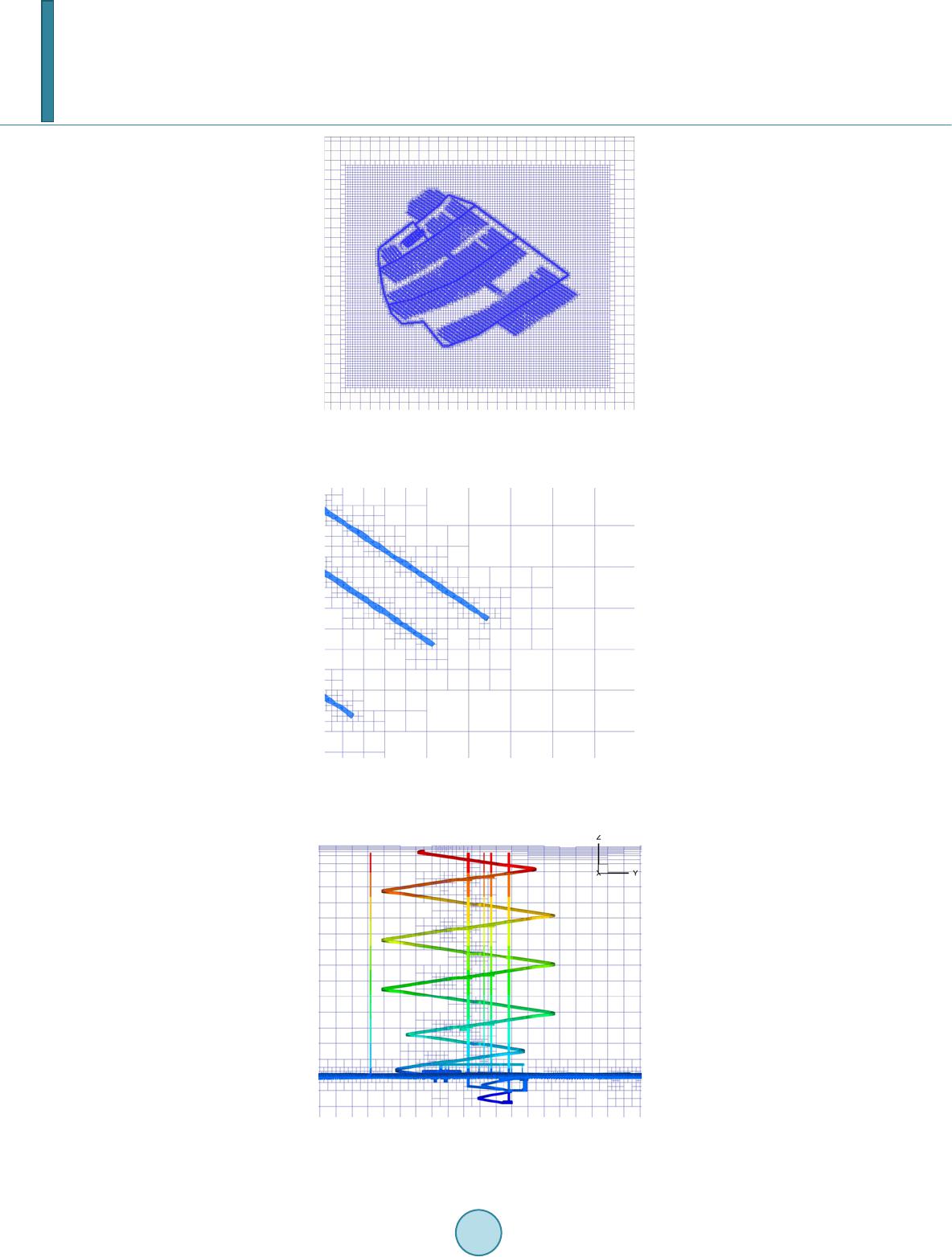

U. Svensson, M. Ferry
378
Figure 10. Plan view of the computational grid at
−465 m elevation. The discretisation around the repo-
sitory was refined using an unstructured grid.
Figure 11. Enlargement showing the discretisation of
the eastern corner of the repository. The size of the
smallest grid cells is 4 m.
Figure 12. Vertical cross-section (South-North) through
the simulated repository. The y-axis points towards north.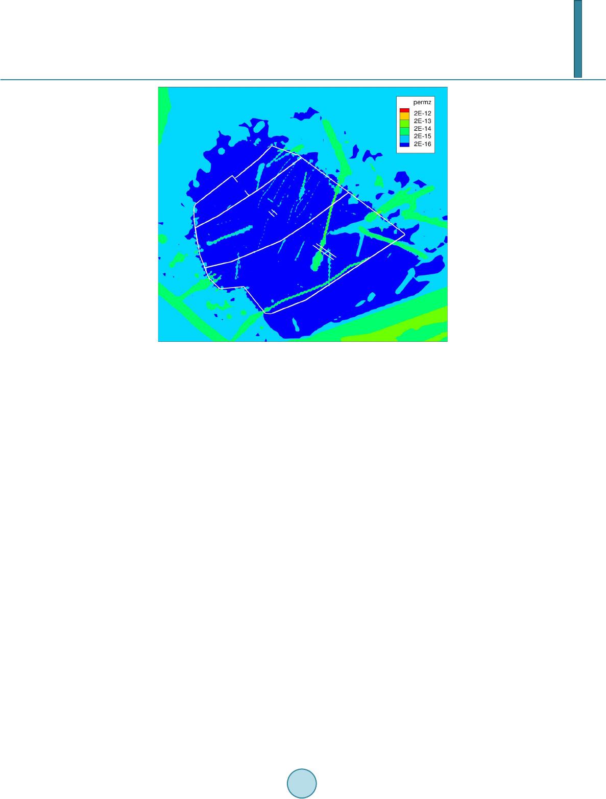

U. Svensson, M. Ferry
379
Figure 13. Plan view of the grid cell vertical permeability field in the target
area at −465 m elevation. The white lines represent the main tunnels.
7.3. Flow Simulations
The inflow simulations during the excavation and operation phases were done in a transient mode for the three
operation stages A-C (Figure 8) and three levels of grouting efficiency I-III (Table 3). Table 4 summarizes the
calculated inflows to the different parts of the repository. The total inflow varied in the range of 7 to 52 L/s (600
to 4600 m3/d), depending on which stage and level of grouting efficiency that is considered.
An illustration of the inflow distribution is given by Figure 14, which represents operation stage C, i.e., the
last one of the three operation stages and grouting level II. Operation stage C rendered the largest inflows. For
the sake of visualization, cells in contact with the repository walls are marked up with spheres if the inflow ex-
ceeded two specified thresholds, 0.1 and 0.5 L/min.
The following two features in F igure 14 are worth noting:
• The ramp seems to have concentrated inflows in its upper part. A part of the simulated inflows to the ramp
may be associated with the intersection with the modelled sheet joints which have a very high transmissivity.
Note also that transport tunnels and ventilation shafts are open.
• Large inflows at repository depth during operation stage C are predominantly encountered along two lines.
This can be explained by the permeability distribution (F igure 13).
8. Discussion
In the introduction it was argued that the computational grid employed by DarcyTools is a strong feature of the
code. In this section this point will be elaborated by an illustration of the cell removal feature. Due to the
sparsely fractured rock, many computational cells are not in contact with a fracture and these cells may in many
cases be removed; often 70% of the cells can be removed. Without increasing the total simulation time, one can
then improve the resolution in other areas.
Figures 15-17 show a grid for the Forsmark repository, where cells not crossed by a fracture have been re-
moved and the resolution close to deposition holes have been increased. Figure 15 should be compared with
Figure 10. White areas in Figure 15 represent areas where grid cells have been removed. Figure 16 gives a
clearer view of how cells are refined close to deposition tunnels. The smallest cell size in the grid is 0.5 m,
which resolves inflows to deposition holes with good resolution, see Figure 17. It should be noted that these
small cells are part of a computational domain of about 10 × 10 × 1 km3 (Figure 9) in a seamless way.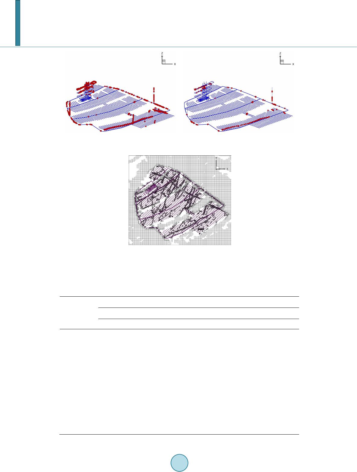

U. Svensson, M. Ferry
380
Figure 14. Cells with an inflow rate greater than 0.1 L/min (top) and 0.5 L/min (bottom) are marked up by
spheres. Operating stage C and grouting level II.
Figure 15. Computational grid for the site scale
at −465 m elevation.
Table 4. Calculated inflow rates (L/s) to different parts of a final repository at Forsmark for three levels of
grouting efficiency, I-III, and three stages of operation, A-C. The three operation stages were run in sequence,
where stage A lasted for 15 years, stage B lasted for 15 years and stage C lasted for 20 years. CA = central
area, DA = deposition area, MT = transportation and main tunnels and VS = ventilation shaft.
Part of
repository
Grouting level I Grouting level II Grouting level III
Operation stage Operation stage Operation stage
A B C A B C A B C
CA-part 1
CA-part 2
CA-part 3
CA-part 4
1
0
3
0
1
0
3
0
2
0
3
0
1
0
1
0
1
0
1
0
1
0
1
0
0
0
1
0
0
0
1
0
0
0
1
0
DA
6
–
–
–
8
–
–
–
9
4
–
–
–
6
–
–
–
8
3
–
–
–
3
–
–
–
4
RAMP-part 1
RAMP-part 2
13
3
14
3
14
3
5
1
5
1
5
1
2
0
2
0
2
0
MT
6
–
–
6
1
–
7
1
9
4
–
–
4
1
–
5
1
5
2
–
–
2
0
–
2
0
2
VS1
VS2
1
–
1
2
1
2
1
–
1
1
0
1
0
–
0
0
0
0
Total 33 39 51 17 21 28 8 8 11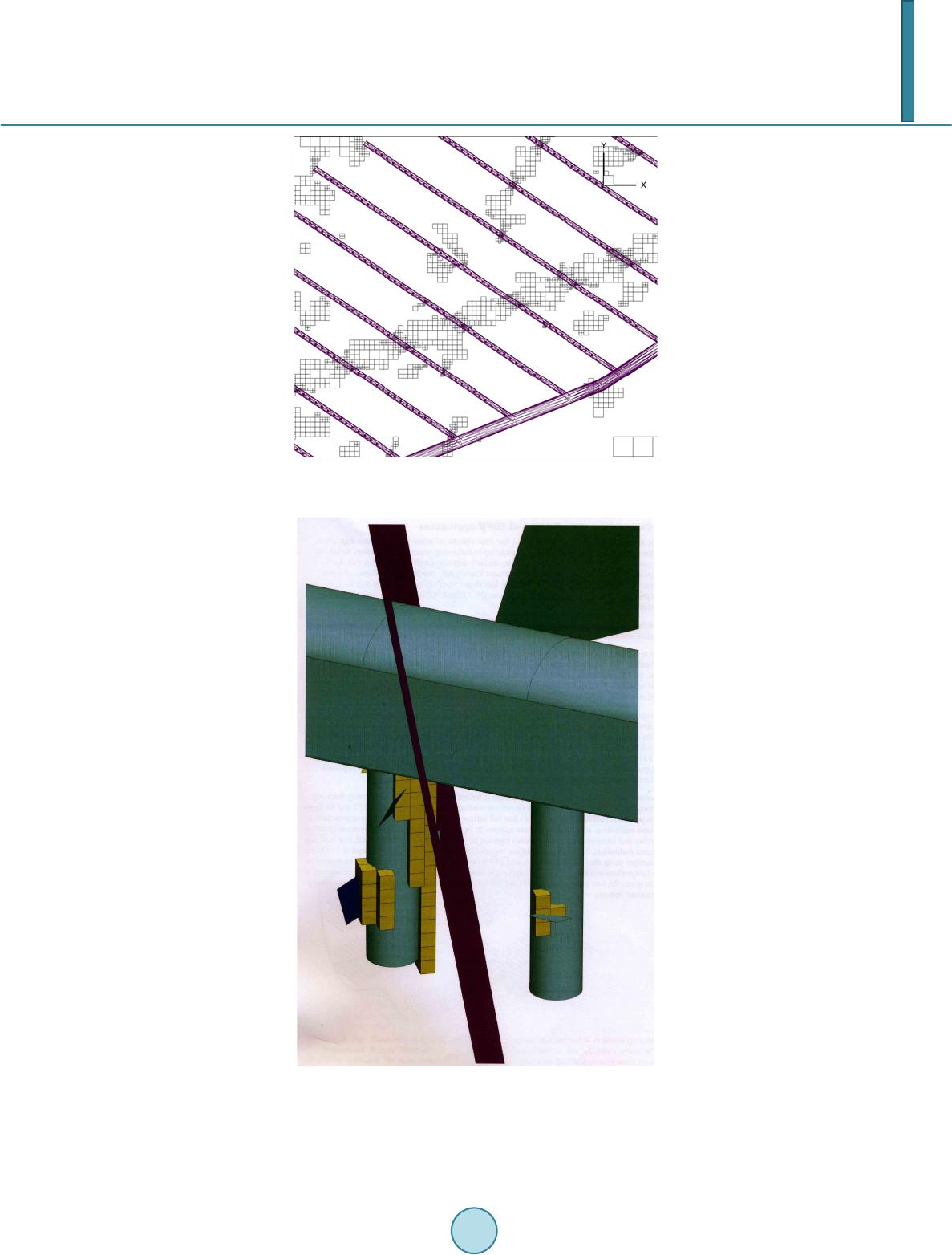

U. Svensson, M. Ferry
381
Figure 16. Computational grid for deposition tunnel scale.
Also the CAD grid for the repository is shown, for orientation.
Figure 17. Illustration of computational cells in contact with
two deposition holes. Also the centre plane of some fractures
are shown. The thickness of all fractures was here set to one
metre and the computational cells shown are for this reason in
contact with the fractures shown.

U. Svensson, M. Ferry
382
The solvers, described in Section 5, are developed to handle these kinds of grids in an efficient manner; in-
cluding the SPMD parallelization.
9. Concluding Remarks
A computer code can be designed in various ways, depending on the intended use and the intended user. A code
that has a single well defined task will normally put less demand on the user. On the other hand, a code that al-
lows for new equations to be introduced, complex boundary conditions, new source terms, etc will require a
deeper understanding from the user. DarcyTools belongs to the latter category. A user should be able to solve a
wide range of problems (1D, 2D and 3D, steady/transient, from µm to km, any kind of boundary condition, arbi-
trary number of advection/diffusion equations, density stratification, fractured or porous media and more). For
this reason, DarcyTools is more of an equation solver than a specific problem solver.
Development is, generally speaking, governed by the demands from applications (see Table 2). This devel-
opment started about 12 years ago and features have been introduced successively since then. Presently devel-
opments follow two parallel lines:
• The present version is considered to fulfil most of the demands from the present range of applications. De-
velopment is hence directed towards refinement, efficiency and confidence building.
• The next major release will introduce a Navier-Stokes solver. One example of a possible application is flow
and transport in a single rock fracture. Such a model can be used to study dispersion at a fracture crossing or
for simulating the grouting process. Also turbulent flows (Reynolds equation and advanced turbulence mod-
els) will be within scope. Flow beneath an ice sheet is one application in mind, another flow and transport in
lakes and rivers (coupled with the groundwater flow).
In addition to the demands from applications, a computer code needs to be continuously developed to make
best use of the computer hardware, new solver techniques and developments in programming.
Acknowledgements
The authors are grateful to the Swedish Nuclear Fuel and Waste Management Company (SKB) for supporting
the writing of the paper. Also the free use of DarcyTools, owned by SKB, is acknowledged.
References
[1] Jackson , C.P., Andrew, R.H. and Todman, S. (2000) Self-Consistency of Heterogeneous Continuum Porous Medium
Representation of a Fractured Medium. Water Resources Research, 36, 189-202.
http://dx.doi.org/10.1029/1999WR900249
[2] Sahimi, M. (19 95 ) Flow and Transport in Porous Media and Fractured Rock: From Classical Methods to Modern Ap-
proach es. VCH. , Weinh eim, 482pp.
[3] Hartley, L. an d Jo yce, S. (2013) Approaches and Algorithms for Groundwater Flow Modeling in Support of Site Inves-
tigations and Safety Assessment of the Forsmark Site, Sweden. Journal of Hydrology.
[4] Svensso n, U., Ferry, M. and Kuylenstierna, H.-O. (2010 ) D arcyTool s, Version 3.4. Concepts, Methods and Equations.
SKB R-10-70, Svensk Kärnbränslehantering AB. 144pp.
[5] Svensso n, U. and Ferry, M. (2010 ) DarcyTools, Version 3.4. User’s Guide. SKB R-10-72, Svensk Kärnbränslehanter-
ing AB.
[6] Svensso n, U. (2010 ) DarcyToo ls, Version 3.4. Verification, Validation and Demonstration. 2010, SKB R-10-71,
Svensk Kärnbränslehantering AB.
[7] Pru es s , K. (1991 ) TOUGH2 a General-Purpose Numerical Simulator for Multiphase Fluid and Heat Flow. Report,
LBN L-29400, Lawrence Berkeley Laboratory, Berkeley, Ca.
[8] McDo nal d, M.G. and Harbaugh, A.W. (1988) A Modular Three-Dimensional Finite-Difference Ground-Water Flow
Model. 1988, U.S. Geol. Surv. Tech. Water Resour. Invest. Book 6, Chap. 2.
[9] Hammond, G.E. and Lichtner, P.C. (2010) F i eld-Scale Model for the Natural Attenuation of Uranium at the Hanford
Area Using High-Performance Computing. Water Resources Research, 46, WO9527.
http://dx.doi.org/10.1029/2009WR008819
[10] Dershowitz, W., Lee, G., Geier, J., Foxford, T. and Ahlstrom, E. (1999) FracMan Interactive Discrete Feature Data
Analysis, Geometric Modeling, and Exploration Simulation. User Documentation, Version 2.6, Golder Associates Inc.

U. Svensson, M. Ferry
383
[11] Bian , H.B., Jia, Y., Amand, G., Duveau, G. and Sh ao, J.F. (2012) 3D Numerical Modeling Thermo-Hydromechanical
Behavior of Underground Storages in Clay Rock. Tunnelling and Underground Space Technology, 30, 93 -109.
http://dx.doi.org/10.1016/j.tust.2012.02.011
[12] Haggert y, R. and Gorelick, S.M. (1995) Multiple-Rate Mass Transfer for Modeling Diffusion and Surface Reaction in
Media with Pore-Scale Heterogeneity. Water Resources Research, 31, 2383-2400.
http://dx.doi.org/10.1029/95WR10583
[13] Svensson , U. (2001) A Continuum Representation of Fracture Networks. Part I: Method and Basic Test Cases. Journal
of Hydrology, 250, 170-186. http://dx.doi.org/10.1016/S0022-1694(01 )0 0435 -8
[14] Svensson , U. (2001) A Continuum Representation of Fracture Networks. Part II: Application to the Äspö Hard Rock
Laboratory. Journal of Hydrology, 250 , 187 -205. http://dx.doi.org/10.1016/S0022-1694(01)00436-X
[15] Diskin, B., Thomas, J.L., Nielsen, E.J., Nishikawa, H. and White, J.A. (2010) Comparison of Node-Centered and Cell-
Centered Unstructured Finite-Volume Discretizations: Viscous Fluxes. American Institute of Aeronautics and Astro-
nautics, 48.
[16] Spalding, D.B. (19 72) A Novel Finite Difference Formulation for Differential Expressions Involving Both First and
Second Derivatives. I ntern ational Journal for Numerical Methods in Engineering, 4, 551-559.
http://dx.doi.org/10.1002/nme.1620040409
[17] Roach e, P.J. (1976) Computational Fluid Dynamics. Hermosa Publs., Albuquerque, 446pp.
[18] Aftosmis, M.J., Berger, M.J. and Mel to n , J.E. (1999) Adaptive Cartesian Mesh Generation. In: Thompson, J.F., Soni,
B.K. and Weatherill, N .P., Ed s., Handbook of Grid Generation, CRC Press, Boca Raton, 1136 pp .
[19] Saad , Y. and Schultz, M.H. (1996) GMRES: A Generalized Minimal Residual Algorithm for Solving Nonsymmetric
Linear Systems. SIAM Journal of Scientific and Statistical Computing, 7, 856-869.
[20] Stüben, K. and Trottenb erg, U. (1982) Multigrid Methods: Fundamental Algorithms, Model Problem Analysis and
Applications. Multigrid Methods, Lecture Notes in Mathematics, 960 , 176.
[21] Stüben, K. (2001) Algebraic Multigrid (AMG): An Introduction with Applications. In: Trot tenberg, U., Oosterlee, C.
and S chüller , A., Eds., Multi g rid, Academic Press, London,
[22] Ferry, M. (2002) New Features of MIGAL Solver. 9th International PHOENICS Users Conferen ce, Moscow.
[23] Aftosmis, M.J., Berger, M .J. and Mu rman, S.M. (2004) Applications of Space-Filling Curves to Cartesian Methods for
CFD. 42nd AIAA, Aerospace Sciences Meeting and Exhibition, Chapter.
[24] Sagan, H. (1994) Space Filling Curves. Springer-Verlag, 193pp. http://dx.doi.org/10.1007/978-1-4612-0871-6
[25] Selroos, J-O. and Follin, S. (201 0 ) SR-Site Groundwater Flow Modeling Methodology, Setup and Results. SKB
R-09-22, Svensk Kärnbränslehantering AB. 125pp.
[26] Vidstrand, P., Follin, S. and Zugec , N. (2010) Groundwater Flow Modeling of Periods with Periglacial and Glacial
Climate Conditions—Forsmark. SKB R-09-21, 190pp, Svensk Kärnbränslehantering AB.
[27] Svensson , U. and Follin, S. (2010) Groundwater Flow Modelling of the Excavation and Operational Phases—Fo rsmark.
SKB R-09-19, Svensk Kärnbränslehantering AB.
[28] Joyce , S., Applegate, D., Hartley, L., Hoek, J., Simpson, T., Swan, D. and Marsic, N, (2010) Groundwater Flow Mod-
elling of Periods with Temperate Climate Conditions—SR-Site Forsmark. SKB R-09-20, 2010, Svensk Kärnbränsle-
hantering AB.