Journal of Intelligent Learning Systems and Applications, 2011, 3, 57-69
doi:10.4236/jilsa.2011.32008 Published Online May 2011 (http://www.SciRP.org/journal/jilsa)
57
An Artificial Neural Network Model to Forecast
Exchange Rates#
Vincenzo Pacelli1*, Vitoantonio Bevilacqua2, Michele Azzollini3
1Faculty of Economics, University of Foggia, Foggia, Italy; 21st Faculty of Engineering—Electrical and Electronic Engineering De-
partment, Polytechnic of Bari, Bari, Italy; 3BancApulia S.p.A., San Severo, Italy.
Received July 10th, 2010; revised October 1st, 2010; accepted December 1st, 2010.
ABSTRACT
For the purposes of this research, the optimal MLP neural network topology has been designed and tested by means the
specific genetic algorith m multi-objective Pareto-Based. The objective of the research is to predict the trend of the ex-
change rate Euro/USD up to three days ahead of last data available. The variable of output of the ANN designed is then
the daily exchange rate Euro/Dollar and the frequency of data collection of variables of input and the output is daily.
By the analysis of the data it is possible to conclude that the ANN model developed can largely predict the trend to
three days of exchange rate Euro/USD.
Keywords: Exchange Rates, Forecasting, Artificial Neural Networks, Financial Markets
1. Introduction
The recent international economic crisis has highlighted
the need for banks to implement effective systems for
estimating risks of market. In particular, the internationa l
activity of the largest banks and the increasing volatility
of exchange rates emphasize the importance of exchange
rate risk, whose active management by the banks require
the use of effective forecasting models.
The study of the topic of forecasting in financial mar-
kets is based on the research hypo theses that:
(h1) the process of pricing in financial markets is not
random;
(h2) the degree of information efficiency at Fama of
the financial markets is not strong or semi-strong.
If the two research hypotheses proposed were not con-
sidered valid, it would be highly redundant and useless to
study the issue of forecasting in financial markets.
If the first hypothesis (h1) was invalid, in fact, it would
assume that the processes of pricing in financial markets
are governed by the random walk model, whereby the
price dynamics are determined by the interaction of an
indefinite variety of interacting causes not modelling and
among them not ordered by relevance. In other words,
we assume that the processes of pricing in financial
markets are governed by the noise. This would make it
useless to study models of forecasting because the case is
not predicta bl e.
If the second hypothesis (h2) was invalid, however, it
would assume that all relevant information are instantly
incorporated in the pricing of financial products, making
essentially unnecessary and economically inconvenient
any efforts to develop models to predict the future based
on present information.
This research aims to analyze the ability of mathe-
matical models of nonlinear nature, such as artificial
neural networks, to highlight non-random and therefore
predictable behaviour in a highly liquid market and
therefore characterized by high efficiency, such as the
exchange rate Euro/US dollar. To this end, it was devel-
oped and empirically tested a non-linear model for fore-
casting exchange rates.
Economic theory has not yet provided econometric
models to produce efficient forecasts of exchange rates,
although many studies have been devoted to the estima-
tion of equilibrium of ex change rates, including:
1) Cassel [1], Samuelson [2], Frankel [3], MacDonald
[4], Alba and Papell [5], Alba and Park [6], Coacley,
Flood, Fuertes and Taylor [7], Kim B.H., Kim H.K. and
Oh [8], Taylor [9], Grossmann, Simpson and Brown [10]
on the theory of Purchasing Power Parity (PPP);
#Although the research has been conducted jointly by the three authors,
p
aragraphs 1, 2 and 7 can be attributed to Vincenzo Pacelli, paragraph
5 is due to Vitoantonio Bevilacqua, while paragraphs 3, 4 and 6 are a
collaborative effort of the three authors.

An Artificial Neural Network Model to Forecast Exchange Rates 58
2) Mundell [11], Dornbusch [12,13], Frenkel [14],
Frenkel and Mussa [15], Rogoff [16] on the monetary
approach;
3) Branson [17], Branson and Henderson [18], Allen
and Kenen [19], Cifarelli and Paladino [20] on the ap-
proach of financial assets or balance of the portfolio.
Despite significant advances in econometric theory on
the estimation of exchange rates, empirical results emerg-
ing from many studies, among others, Frankel [21] and
Froot and Rogoff [22] to refute the theory of purchasing
power parity; Frankel [23] against the monetary model,
Branson, Halttunen and Masson [24] and Frenkel [25] to
refute the theory of financial assets do not provide spe-
cial support to the theories mentioned, except in the long
term.
In particular, Meese and Rogoff [26] found that none
of the forecasting models of the exchange rate estab-
lished by economic theory has a better abilit y to forecast,
over a period lower than 12 months, rather than the for-
ward rate models or random walk, emphasizing the pa-
radox that the variations of exchange rates are com-
pletely random. In the wake of the study of Meese and
Rogoff [26], some authors, including Hsieh [27], Vas-
silicos, Demos, Tata [28], Leroy, Nottola [29], Refenes,
Azema Barac, Chen, Karoussos [30], Nabney, Dunis,
Dallaway, Leong, Redshaw [31,32], Brooks [33], Tenti
[34], Dersch, Flower, Pickard [35], Lawrence, Giles,
Tsoi [36], Rauscher [37], El Shazly MR, El Shazly HE
[38], Gabbi [39], Gencay [40], Soofi, Cao [41], Sarno
[42], Alvarez and Alvarez-Diaz [43-45] Alvarez-Diaz
[46], Reitz and Taylor [47], Anastakis and Mort [48],
Majhi, Panda and Sahoo [49], Bereau, Lopez and Vil-
lavicencio [50], Norman [51], Bildirici, Alp and Ersen
[52], have studied the predictability of the dynamics of
exchange rates of non-linear models such as neural net-
works, genetic algorithms, expert systems or fuzzy mod-
els, leading however to conflicting results.
It is unnecessary to underline that the theme of fore-
casting in financial markets is not confined to the specific
case of foreign exchange markets, but it is extended to all
financial assets. This is because the mechanisms that
determine and influence the pricing in financial markets
are still largely unknown, although many studies have
been devoted over the years at this issue as early as by
Keynes in chapter 12 of Book IV of his The General
Theory of Employment, Interest and Money in March of
1936 [53]. After Keynes, some authors (Meese and Ro-
goff [26]; Schiller [54]; Soros [55], Obstfeld and Rogoff,
[56]; Rogoff [57]) have highlighted the inability of eco-
nomic theory to unravel the mechanisms that determine
price movements in financial markets, highlighting the
inadequacy for th e purpose of both models of fundamen-
tal analysis and technical one.
In general, the prediction of financial time series re-
quires the prior identification of a specific portfolio of
variables (input data for forecasting models) which are
explanatory of the phenomenon to be foreseen and
therefore significantly influence the pricing (output for
forecasting models). The forecasting models, in fact, will
learn the characteristics of the phenomenon to be fore-
seen by the variables of input selected and by historical
data that represent the phenomenon analyzed. Models
predicting the financial phenomena, developed by eco-
nomic theory over the years, can be classified into two
main categories:
 structural prediction models or linear ones, such as
econometric models as Autoregressive Conditional
Heteroschedasticity (ARCH), Generalized Autore-
gressive Conditional Heteroschedasticity (GARCH),
State Space, which are based on the general view
that every action of traders can be explained by a
model of behaviour and thus by a definite, explicit
function that can bind variables determinants of the
phenomenon to be fo re seen;
 black box forecasting models or non-linear ones,
such as neural networks, genetic algorithms, expert
systems or fuzzy models, which, through the learn-
ing of the problem analyzed, attempting to identify
and predict the non random and non-linear dynam-
ics of prices, but without explicit ties and logical
functions that bind the variables analyzed.
This paper will deepen in particular the second class of
forecasting models, through the development and em-
pirical application of a neural network model for fore-
casting the exchange rate EUR/USD for up to three days
ahead of last data available.
2. A Literature Review
The literature on the application of artificial intelligence
systems (such as neural networks, expert systems, fuzzy
models and genetic algorithms) to the fields of econom-
ics and finance has explored various aspects. In particular
lots of studies have analyzed the application of these
models on time series forecasting.
Over the years, the literature has produ ced several stu-
dies to highlight both the critical factors and point of
strengths of artificial intelligence models in the forecast-
ing of financial phenomena and to propose tools to fa-
cilitate trading in financial markets.
Among the most significant contributions we can
mention Yu and Bang [58], Zhang, Patuwo and Hu [59],
Kashei, Hejazi and Bijari [60], Wong, Xia and Chu [ 61],
Yu and Huarng [62].
In the paper of H. Y. Yu and S. Y. Bang [58], the au-
thors develop a new learning algorithm for the FIR neu-

An Artificial Neural Network Model to Forecast Exchange Rates59
ral network model by applying the idea of the optimiza-
tion layer by layer to the model. The results of the ex-
periment, using two popular time series prediction prob-
lems, show that the new algorithm is far better in learn-
ing time and more accurate in prediction performance
than the original learning algorithm. The FIR neural
network model can be proposed for time series prediction
giving good results. However, the learning algorithm
used for the FIR network is a kind of gradient descent
method and hence inherits all the well-known problems
of the method.
G. P. Zhang, B. E. Patuwo and M. Y. Hu [59] presents
an experimental evaluation of neural networks for nonli-
near time-series forecasting. The effects of three main
factors (input nodes, hidden nodes and sample size) are
examined through a simulated computer experiment.
Results show that neural networks are valuable tools for
modelling and forecasting nonlinear time series while
traditional linear methods are not as competent for this
task. The number of input nod es is much more important
than the number of hidden nodes in neural network mod-
el building for forecasting. Moreover, large sample is
helpful to ease the over fitting problem.
In the paper of M. Khashei, S. R. Hejazi and M. Bijari
[60], based on the basic concepts of ANNs and fuzzy
regression models, a new hybrid method is proposed that
yields more accurate results with incomplete data sets. In
their proposed model, th e advantages of ANNs and fuzzy
regression are combined to overcome the limitations in
both ANNs and fuzzy regression models. The empirical
results of financial market forecasting indicate that the
proposed model can be an effective way of improving
forecasting accuracy.
In the study of W. K. Wong, M. Xia and W. C. Chu
[61], a novel adaptive neural network (ADNN) with the
adaptive metrics of inputs and a new mechanism for ad-
mixture of outputs is proposed for time-series prediction.
The adaptive metrics of inpu ts can solve the problems of
amplitude changing and trend determination, and avoid
the over-fitting of networks. The new mechanism for
admixture of outputs can adjust forecasting results by the
relative error and make them more accurate. The pro-
posed ADNN method can predict periodical time-series
with a complicated structure. The experimental results
show that the proposed model outperforms the auto-re-
gression (AR), artificial neural network (ANN), and
adaptive k-nearest neighbors (AKN) models. The ADNN
model is proved to benefit from the merits of the ANN
and the AKN through its’ novel structure with high ro-
bustness particularly for both chaotic and real ti me-series
predictions.
The paper of T. H. K. Yu and K. H. Huarng [62] in-
tends to apply neural networks to implement a new fuzzy
time series model to improve forecasting. Differing from
previous studies, this study includes the various degrees
of membership in establishing fuzzy relationships, which
assist in capturing the relationships more properly. These
fuzzy relationships are then used to forecast the stock
index in Taiwan. This study performs out-of-sample fo-
recasting and the results are compared with those of pre-
vious studies to demonstrate the performance of the pro-
posed model.
3. The Construction of the Data Base
The construction of the data base used to train the artifi-
cial neural network (ANN) developed was divided into
the following three phases:
 data collection;
 data analysis;
 variable selection.
The phase of data collection must achieve the follow-
ing objectives:
 regularity in the frequency of the data collection by
the markets;
 homogeneity between the information provided to
the ANN and that available for the market opera-
tors.
In the phase of the data collection, we were, therefore,
initially considered, as variables of input, both macro-
economic variables (fundamental data) and market data,
from which it was assumed that the behaviour of the ex-
change rate euro-dollar was conditional. The data were
collected from January 1999 to December 31, 20091. The
variables of input are listed in the Table 1, ind icating the
frequency of the data collection and the acronyms of va-
riables used in the tables of the similarity matrix.
Once collected all the data, we moved to the stage of
their analysis, which aims to select the data that will be
used to train ANN among those initially collected. This
phase is crucial, because the learning capacity of the
ANN depends on the quality of information provided,
which is the capacity of this information to prov ide a true
representation of the phenomenon without producing
ambiguous, distorting or amplifying effects in the phases
of training networks.
In this phase, the observation of the correlation or si-
milarity coefficients (shown below in Tables 2 and 3)
allow to evaluate the nature of relations between the va-
riables of input consider ed, suggesting the elimination of
the variables highly correlated with each other and
therefore capable to product amplifying or distorting ef-
fects during the training phases.
Tables 2 and 3 show, respectively, the coefficients of
1Source of data ar e Bloomberg and Borsa Italiana.

An Artificial Neural Network Model to Forecast Exchange Rates 60
Table 1. Variables of input initially selected. correlation or similarity of the daily and monthly initial
variables.
Variables Frequency
Dow Jones Euro Stoxx 50 Index Daily
FTSE 100 Index Daily
National Association of Securities Dealers Automated
Quotation - Nasdaq Composite Index (NASDAQ) Daily
Cotation Assistée en Continu – CAC 40 index (CAC) Daily
Deutscher Aktien Index (DAX) Daily
Dow Jones Industrial Average (DOW JONES) Daily
Standard and Poor’s 500 Index (SP) Daily
Exchange Rate EUR/GBP (GBP) Daily
Exchange Rate EUR/YEN (YEN) Daily
Exchange Rate EUR/USD (USD) Daily
Exchange Rate EUR/NZD (NZD) Daily
Gold Spot Price USA (GOLDS) Daily
Silver Spot Price USA (SILV) Daily
Oil Price (CLA) Daily
Natural Gas Accounts (NGA) Daily
LIBOR Rate 3m $ (L3M) Daily
EURIBOR Rate 3M € (EU3M) Daily
Avarage yield on Government Bond to 2 years in U.S.
area (usgg2yr) Daily
Avarage yield on Government Bond to 5 years in U.S.
area (usgg5yr) Daily
Avarage yield o n Government Bond to 5 years in
Eurozone (gecu5yr) Daily
Avarage yield o n Government Bond to 2 years in
Eurozone (gecu2yr) Daily
Monetary Aggregate M1 USA $ (M1$YOY) Monthly
Monetary Aggregate M2 USA $ (M2$YOY) Monthly
Monetary Aggregate M1 Euro € (M1€ YOY) Monthly
Monetary Aggregate M2 Euro € (M2€ YOY) Monthly
Consumer Price Indices Euro a/a (ECCPEMUY) Monthly
Consumer Price Indices USA a/a (CPI YOY) Monthly
Eur Trade Balance (XTSBEZ) Monthly
USA Trade Balance (USTBTOT) Monthly
Eur Consumer Confidence (EUCCEMU) Monthly
USA Consumer Confidence (CONCCONF) Monthly
Eur Investor Confidence (EUBCI) Monthly
Eur Industrial Confidence (EUICEMU) Monthly
Eur Unemployment Rate (UMRTEMU) Monthly
USA Unemployment Rate (USURTOT) Monthly
Eurostat Eurozone Monthly Product ion in Construction
SA (EUPREMU) Monthly
USA Index of real estate - Nahb Stati Uniti
(USHBMIDX) Monthly
USA Retail Sales (RSTAMOM) Monthly
USA Government Debt (DEBPTOTL) Monthly
Eur Industri a l Production (EUIPEMUY) Monthly
USA Industrial Production (IP YOY) Monthly
Deficit/surplus % Pil USA (FDDSGDP) Monthly
Following the analysis of the correlation coefficients,
we moved to the stage of selection of variables and we
eliminated the variables with the following characteris-
tics:
 variables characterized by a Pearson correlation
coefficient with at least one other variable consid-
ered above the threshold level of acceptance equal
to 0.802;
 monthly variables, because, having developed a
neural network with a daily frequency of data col-
lection of variables of input and output, they were
considered potentially able to produce ambiguous
or redundant signals during the training of ANN.
As a result of the selection of variables conducted ac-
cording to the criteria outlined above, we have the final
set of seven input variables to train the neural network,
which is in the next section . In establishing the final data
set with data of the seven input variables, exceptional
values, as the outliers, were also removed related to spe-
cial historical events such as the terrorist attacks of Sep-
tember 11, 2001.
4. The Methodology for the Development of
the Artificial Neural Network Model
The objective of the ANN is to predict the trend of the
exchange rate Euro/USD up to three days ahead of last
data available. The variable of output of the ANN de-
signed is then the daily exchange rate Euro/Dollar and
the frequency of data collection of variables of inpu t and
the output is daily.
In drawing up the network it was considered that the
exchange rate is characterized by the so-called phe-
nomenon of mean reversion3, or by the tendency not to
maintain a trend up or down for a long time4.
As noted in paragraph 3, as a result of the processing
steps of the data base, we have selected the following
even variables of input of the ANN. s
2Since the coefficient of correlation or similarity between two variables
analyzed both at the time “t”is merely indicate what the change of a
variable “x” is similar to the change of a variable “y”, which follow the
same trend, it was considered necessary to eliminate the variables most
strongly correlated with each other in order to avoid potentially am-
b
iguous or amplifying signals in the stages of training. The fact o
f
considering as input of a neural network two or more variables strongly
correlated (i.e. Pearson’s coefficient > 0.80), would artificially boost
the information provided by the neural network variables in question.
3See Gabbi (1999) , pag. 241.
4Empirical evidence shows that exchange rates tend to remain suffi-
ciently stable in the medium term around a mean value of equilibrium.
It occurs that too high values compared with the average period reflect
a tendency to return later to the media. The prediction of these vari-
ables, therefore, may be affected by distorting effects produced by
historical dynamic, as the typical behaviour of the series is precisely to
reverse the trend.

An Artificial Neural Network Model to Forecast Exchange Rates 61
Table 2. Similarity matrix of daily variables.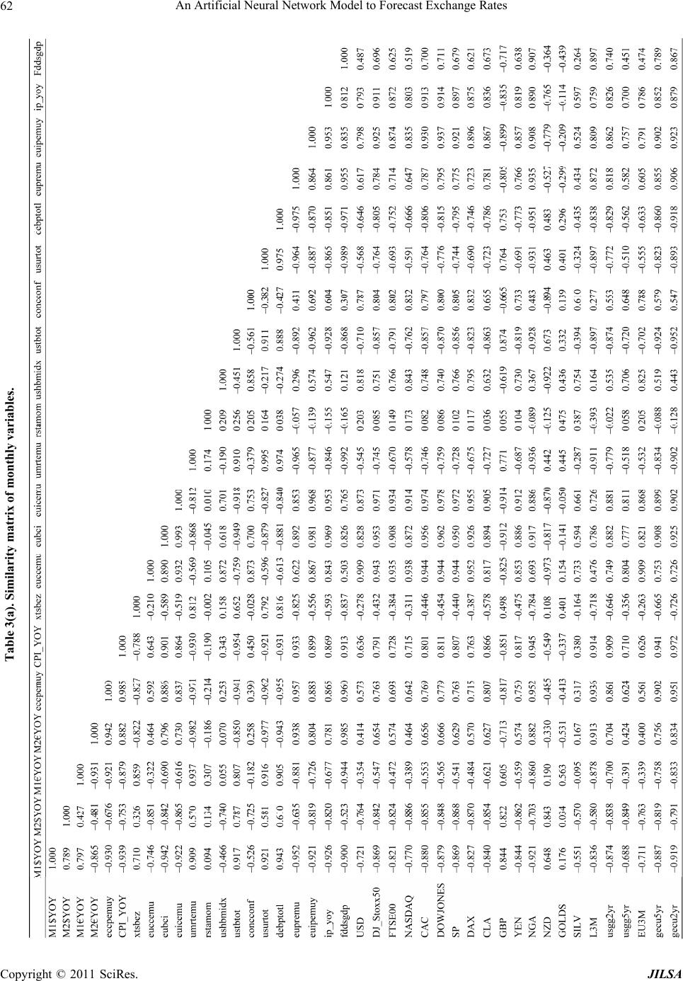

An Artificial Neural Network Model to Forecast Exchange Rates 62
Table 3(a). Similarity matrix of monthly variables.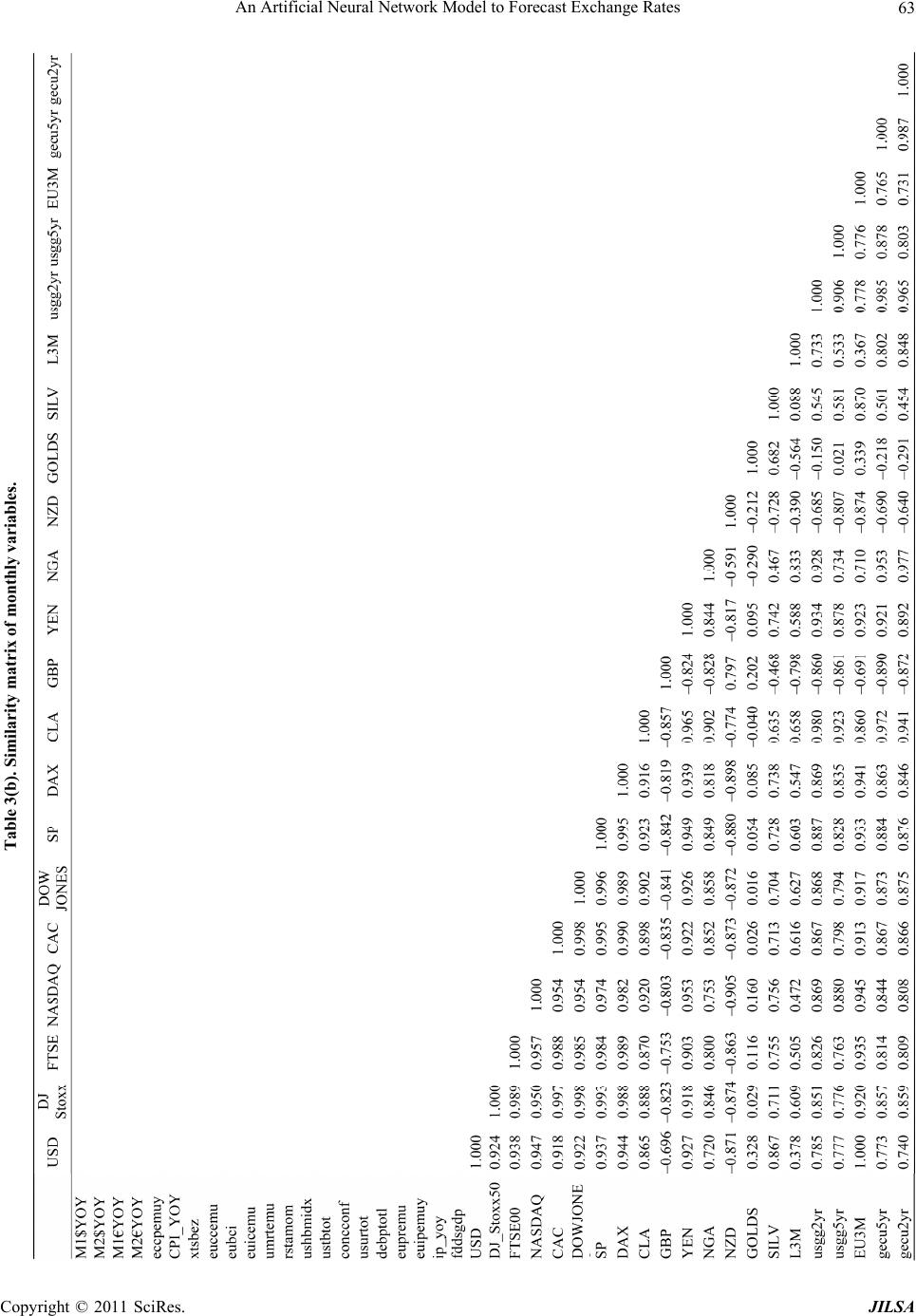

An Artificial Neural Network Model to Forecast Exchange Rates 63
Table 3(b). Similarity matrix of monthly variables.

An Artificial Neural Network Model to Forecast Exchange Rates 64
 Nasdaq Index;
 Daily Exchange Rate Eur/USD New Zeland;
 Gold Spot Price USA;
 Average returns of Government Bonds—5 years
in the USA zone;
 Average returns of Government Bonds—5 years in
the Eurozone;
 Crude Oil Price—CLA (Crude oil);
 Exchange rate Euro/US dollar of the previous day
compared to the day of the output.
For each of these variables of input historical memory
was calculated, which is the number of daily observa-
tions in which it is very h igh the possibility that th e daily
value of the variables is self-correlated with the values of
n days5.
The historical memory was calculated by an polyno-
mial interpolation with coefficient R2 equal to 0.98 for
90% of cases. The historical memories calculated for
each variable are:
 Nasdaq index: eight surveys;
 Daily exchange rate Euro/NZ Dollar: five surveys;
 Spot price of gold expressed in dollars per ounce:
six surveys;
 Average returns of government bonds—5 years in
the USA: eight surveys;
 Average returns of government bonds—5 years in
the Eurozone: seven surveys;
 The price of crude oi l (CLA): eight survey s ;
 Exchange rate Euro/USD: seven surveys more
output6;
In order to predict the trend of historical memories of
individual variables by determining the angular coeffi-
cients (m), it was used by the software MatLab the func-
tion Polyfit7, whereas for the first experiments a degree
of the polynomial approximation of 18.
Since the ANN uses values between –1 and 1 where it
is used the activation function Tansig9, it was necessary
to normalize data through the interpolation performed
with MatLab assigning values between –1 and 1 to vary
of the value of the angular coefficient (m) produced by
the Polyfit, according to the following summary:
IF 0 <= m <= 0.1 Then value = 0.2
IF 0.1 < m <= 1.1 Then value = 0.4
IF 1.1 < m <= 3.1 Then value = 0.6
IF 3.1 < m <= 7.1 Then value = 0.8
IF m > 7.1 Then value = 1
IF –0.1 <= m < 0 Then value = –0.2
IF –1.1 <= m < –0.1 Then value = –0.4
IF –3.1 <= m < –0.1 Then value = –0.6
IF –7.1 <= m < 3.1 Then value = –0.8
IF m < –7.1 Then value = –1
As shown by the previous scheme, the change of the
angular coefficient determines the change in trend growth
or reduction of the exchange rate Euro/USD USA.
The inputs of the network were reduced by 49 (i.e. 7
input with their historical memories) to 7, while the re-
cords10 are 547.
To optimize the performance of the network we have
reduced the data set to avoid signal of distortion or en-
hancement of some information, using 160 examples of
maximum variance, of which 75% (120 examples) for
training set and 25% (40 samples) for the validation set.
5. Optimal Topology Design Multi Layer
Perceptron Neural (MLP) through a
Multi-Objective Genet ic Algorithm
The problem of finding the optimal topology of a Multi
Layer Perceptron (MLP) neural network as a trade-off
between the performance in terms of precision and the
performance in terms of generalization, avoiding the
problems of overfitting during the training phase, has
been analyzed in the literature very accurately [63] and
described in details in terms of an innovative genetic
algorithm multi-objective Pareto -Based optimization pro-
blems [64] in which a bi-objective functions problems
has been formulated and implemented. In fact decisions
made in the network design ing phase could turn ou t to be
critical and choices non coherent with the problem could
influence negatively learning or generalization ability of
the Intelligent System. In this field evolutionary tech-
niques have proven to be a great support in exploring the
complex spaces that characterize the designing process.
The setup of a neural network can be thought of as an
optimization problem, indeed. The employment of such
techniques appeared to be the optimal method in order to
find a competitive solution.
5The construction of the data set the neural network is based on the
concept of historical memory as the objective of the ANN is to predict
the trend of the exchange rate Euro/Dollar.
6To train the neural network it is considered as current moment t-2 fo
r
each variable, so as to obtain two readings back in order to predict a
trend output rate Eur/U.S. dollar equal to three days.
7Function polyfit: polyfit p = (x, fx, n). The polyfit is a function used fo
r
the construction of polynomial interpolation, where x is the vector that
contains the nodes of the grid, fx is the vector containing the values to
interpolate on the grid nodes, n is the degree of the polynomial interpo-
lation.
8A function polyfit degree of approximation equal to 1 (i.e. n= 1) is a
p
olynomial of first degree which interpolates the data as if making a
linear regression values.
9Hyperbolic tangent sigmoid activation function. Tansig (n) = 2/(1 +
exp(–2 * n)) – 1, where n is the matrix of inputs. The results of a func-
tion Tansig can vary between –1 and 1.
Genetic Algorithms (GAs) are well established bio-
inspired computational optimization approaches with a
wide range of applications that spans from finance to
medicine, inspired by the evolutionist theory explaining
the origin of species. Following what happens in nature,
10A record is a set of values of input variables and output.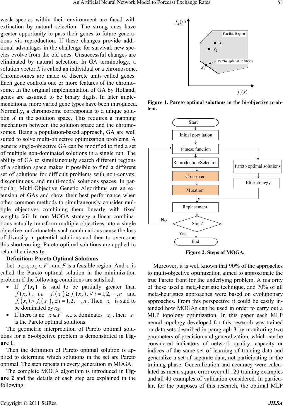

An Artificial Neural Network Model to Forecast Exchange Rates65
weak species within their environment are faced with
extinction by natural selection. The strong ones have
greater opportunity to pass their genes to future genera-
tions via reproduction. If these changes provide addi-
tional advantages in the challenge for survival, new spe-
cies evolve from the old ones. Unsuccessful changes are
eliminated by natural selection. In GA terminology, a
solution vector X is called an individual or a chromosome.
Chromosomes are made of discrete units called genes.
Each gene controls one or more features of the chromo-
some. In the original implementation of GA by Holland,
genes are assumed to be binary digits. In later imple-
mentations, more varied gene types have been introduced.
Normally, a chromosome corresponds to a unique solu-
tion X in the solution space. This requires a mapping
mechanism between the solution space and the chromo-
somes. Being a population-based approach, GA are well
suited to solve multi-objective optimization problems. A
generic single-objective GA can be modified to find a set
of multiple non-dominated solutions in a single run. The
ability of GA to simultaneously search different regions
of a solution space makes it possible to find a different
set of solutions for difficult problems with non-convex,
discontinuous, and multi-modal solutions spaces. In par-
ticular, Multi-Objective Genetic Algorithms are an ex-
tension of GAs and show their best performance when
other common methods to simultaneously consider mul-
tiple objectives combining them linearly with fixed
weights fail. In non MOGA strategy a linear combina-
tions actually transform multiple objectives into a single
objective, unfortunately su ch combinations cau se the loss
of diversity in potential solutions and then to overcome
this shortcoming, Pareto optimal solutions are applied to
retain the diversity.
Definition: Pareto Optimal Solutions
Let 012
,,
x
xx F, and F is a feasible region. And x0 is
called the Pareto optimal solution in the minimization
problem if the following conditions are satisfied.
 If

1
f
x is said to be partially greater than


2
f
x, i.e.
 
12
,1,2,,
ii
f
xfx i

,1,2,, n
and
12ii
 
f
xfxin, Then 1
x
is said to
be domi nated by x2.
 If there is no
x
F s.t. x dominates 0
x
, then 0
x
is the Pareto optimal solutions.
The geometric interpretation of Pareto optimal solu-
tions for a bi-objective problem is demonstrated in Fig-
ure 1.
Then the definition of Pareto optimal solution is ap-
plied to determine which solutions in the set are Pareto
optimal. The step repeats in every generation in MOGA.
The complete MOGA algorithm is introduced in Fig-
ure 2 and the details of each step are explained in the
following.
Pareto Optimal Solutions
.
0
x
.
.
1
x
2
x
)(
2xf
)(
1xf
Feasible Region
Figure 1. Pareto optimal solutions in the bi-objective prob-
lem.
Figure 2. Steps of MOGA.
Moreover, it is well known that 90% of the appro aches
to multi-objective optimization aimed to approximate the
true Pareto front for the underlying problem. A majority
of these used a meta-heuristic technique, and 70% of all
meta-heuristics approaches were based on evolutionary
approaches. From this perspective it could be easily in-
tended how MOGAs can be used in order to carry out a
MLP topology optimization. In this paper each MLP
neural topology developed for this research was trained
on data sets described in paragraph 3 by monitoring two
parameters of precision and generalization, which can be
considered indicators of network quality, capacity or
indices of the same set of learning of training data and
generalize a set of separate data, not participating in the
training phase. Generalization and accuracy were calcu-
lated as mean square error over all 120 training examples
and all 40 examples of validation considered. In particu-
lar, for the purposes of this research, the optimal MLP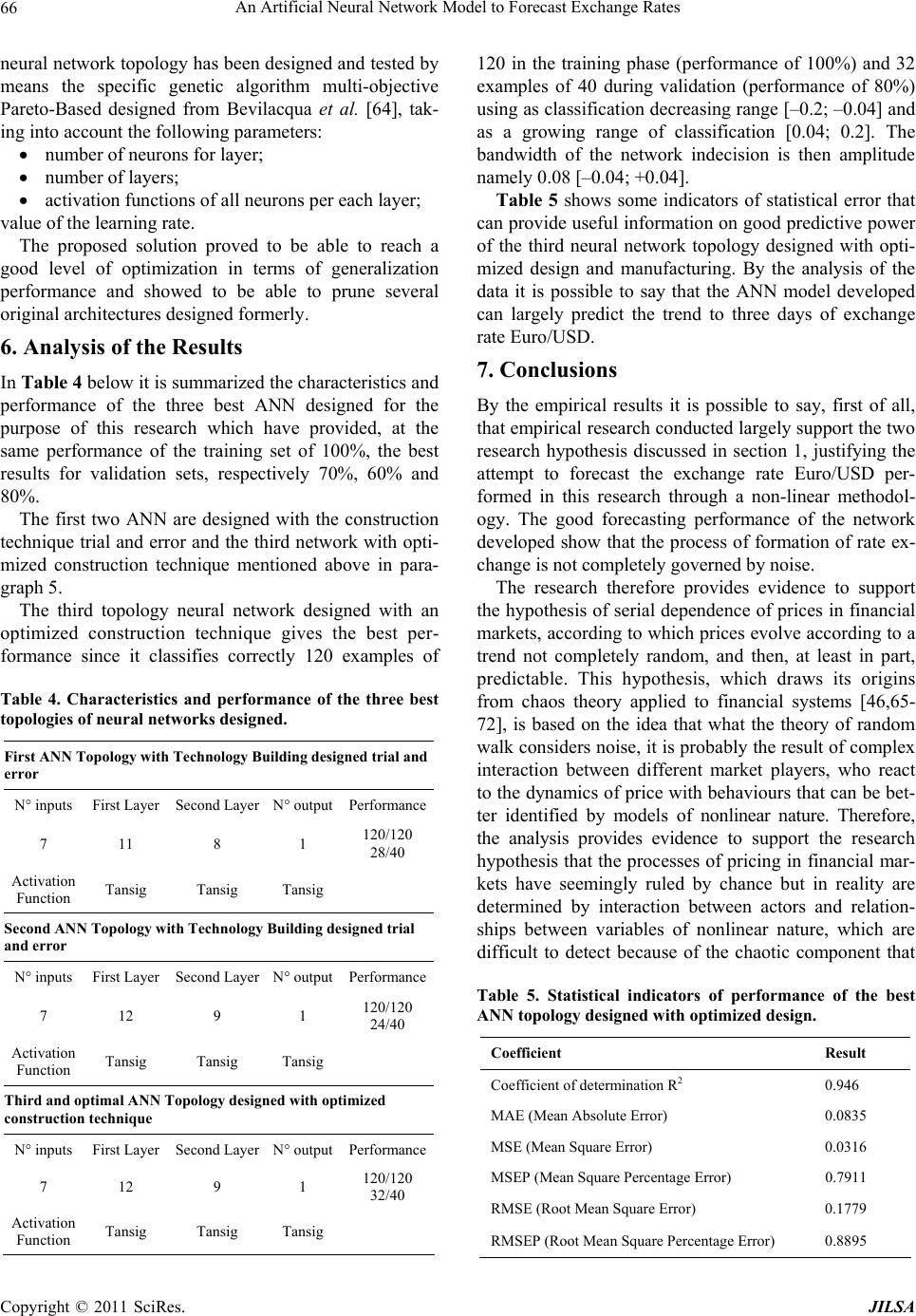

An Artificial Neural Network Model to Forecast Exchange Rates 66
neural network topology has been designed and tested by
means the specific genetic algorithm multi-objective
Pareto-Based designed from Bevilacqua et al. [64], tak-
ing into account the following parameters:
 number of neurons for la y e r ;
 number of layers;
 activation functions of all neurons per each layer;
value of the learning rate.
The proposed solution proved to be able to reach a
good level of optimization in terms of generalization
performance and showed to be able to prune several
original architectures designed formerly.
6. Analysis of the Results
In Tab le 4 below it is summar ized the ch aracteristics and
performance of the three best ANN designed for the
purpose of this research which have provided, at the
same performance of the training set of 100%, the best
results for validation sets, respectively 70%, 60% and
80%.
The first two ANN are designed with the construction
technique trial and error and the third network with opti-
mized construction technique mentioned above in para-
graph 5.
The third topology neural network designed with an
optimized construction technique gives the best per-
formance since it classifies correctly 120 examples of
Table 4. Characteristics and performance of the three best
topologies of neural networks designe d.
First ANN Topology with Technology Building designed trial and
error
N° inputs First Layer Second Layer N° output Performance
7 11 8 1
120/120
28/40
Activation
Function Tansig Tansig Tansig
Second ANN Topology with Technology Building designed trial
and error
N° inputs First Layer Second Layer N° output Performance
7 12 9 1
120/120
24/40
Activation
Function Tansig Tansig Tansig
Third and optimal ANN Topology designed with optimized
construction technique
N° inputs First Layer Second Layer N° output Performance
7 12 9 1
120/120
32/40
Activation
Function Tansig Tansig Tansig
120 in the training phase (performance of 100%) and 32
examples of 40 during validation (performance of 80%)
using as classification decreasing range [–0.2; –0.04] and
as a growing range of classification [0.04; 0.2]. The
bandwidth of the network indecision is then amplitude
namely 0.08 [–0.04; +0.04].
Table 5 shows some indicators of statistical error that
can provide u seful information on go od predictive pow er
of the third neural network topology designed with opti-
mized design and manufacturing. By the analysis of the
data it is possible to say that the ANN model developed
can largely predict the trend to three days of exchange
rate Euro/USD.
7. Conclusions
By the empirical results it is possible to say, first of all,
that empirical research conducted largely sup port the two
research hypothesis discussed in section 1, justifying the
attempt to forecast the exchange rate Euro/USD per-
formed in this research through a non-linear methodol-
ogy. The good forecasting performance of the network
developed show that the process of formation of rate ex-
change is not completely governed by noise.
The research therefore provides evidence to support
the hypothesis of serial dependence of prices in financial
markets, according to which prices evolve according to a
trend not completely random, and then, at least in part,
predictable. This hypothesis, which draws its origins
from chaos theory applied to financial systems [46,65-
72], is based on the idea that what the theory of random
walk considers noise, it is probab ly the result of complex
interaction between different market players, who react
to the dynamics of price with behaviours that can be bet-
ter identified by models of nonlinear nature. Therefore,
the analysis provides evidence to support the research
hypothesis that the processes of pricing in financ ial mar-
kets have seemingly ruled by chance but in reality are
determined by interaction between actors and relation-
ships between variables of nonlinear nature, which are
difficult to detect because of the chaotic component that
Table 5. Statistical indicators of performance of the best
ANN topology designed with optimized design.
Coefficient Result
Coefficient of determination R2 0.946
MAE (Mean Absolute Error) 0.0835
MSE (Mean Square Error) 0.0316
MSEP (Mean Square Percentage Error) 0.7911
RMSE (Root Mean Squ are Error) 0.1779
RMSEP (Root Mean Square Percentage Er ror) 0.8895

An Artificial Neural Network Model to Forecast Exchange Rates67
characterizes the process of pricing in financial markets,
the non-exhaustive information available to build effec-
tive predictive models and the inadequacy of many fore-
casting models. The considerations highlighted above
lead to a final consideration [73], which is essentially
methodological and is about the effectiveness of an inte-
grated approach, which is based on the joint use of linear
and non-linear methods of analysis to study the phe-
nomenon of the forecasting of financial prices.
8. Acknowledgements
The authors acknowledge to the anonymous referees for
their thoughtful and constructive suggestions and Maria
Rosaria Di Muro for the valuable support.
REFERENCES
[1] G. Cassel, “Money and Foreign Exchange 1914,” Mac-
millan, New York, 1923.
[2] P. A. Samuelson, “Theoretical Notes on Trade Problems,”
Review of Economics and Statistics, Vol. 46, No. 2, 1964,
pp. 145-154. doi:10.2307/1928178
[3] J. A. Frankel, “Zen and the Art of Modem Macroeco-
nomics: A Comment ary,” In: W. S. Ha rafat, T. D. Wille t,
Eds., Monetary Policy for a Volatile Global Economy,
American Enterprise Institute for Public Policy Research,
Washington DC, 1990, pp. 117-123.
[4] R. MacDonald, “Exchange Rate Behavior: Are Funda-
mentals Important?” The Economic Journal, Vol. 109, No.
459, 1999, pp. 673-691.
doi:10.1111/1468-0297.00479
[5] J. D. Alba and D. H. Papell, “Purchasing Power Parity
and Country Characteristics: Evidence from Panel Data
Tests,” Journal of Development Economics, Vol. 83, No.
1, May 2007, pp. 240-251.
doi:10.1016/j.jdeveco.2005.09.006
[6] J. D. Alba and D. Park, “Purchasing Power Parity in De-
veloping Countries: Multi-Period Evidence under the
Current Float,” World Development, Vol. 31, No. 12,
December 2003, pp. 2049-2060.
doi:10.1016/j.worlddev.2003.06.008
[7] J. Coakley, R. P. Flood, A. M. Fuertes and M. P. Taylor,
“Purchasing Power Parity and the Theory of General
Relativity: The First Test s,” Journal of International Money
and Finance, Vol. 24, No. 2, March 2005, pp. 293-316.
doi:10.1016/j.jimonfin.2004.12.008
[8] B. H. Kim, H. K. Kim and K. Y. Oh, “The Purchasing
Power Parity of Southeast Asian Currencies: A Time-
Varying Coefficient Approach,” Economic Model ling, Vol.
26, No. 1, January 2009, pp. 96-106.
doi:10.1016/j.econmod.2008.05.009
[9] M. Taylor, “Purchasing Power Parity and Real Exchange
Rates,” Routledge, London, 2009.
[10] A. Grossmann, M. W. Simpson and C. J. Brown, “The
Impact of Deviation from Relative Purchasing Power Par-
ity Equilibrium on U.S. Foreign Direct Investment,” The
Quarterly Review of Economics and Finance, Vol. 49, No.
2, May 2009, pp. 521-550.
doi:10.1016/j.qref.2008.02.001
[11] R. Mundell, “International Economics,” MacMillan, New
York, 1968.
[12] R. Dornbush, “Currency Depreciation, Hoarding and
Relative Prices,” Journal of Political Economy, Vol. 81,
No. 4, 1973, pp. 893-915. doi:10.1086/260087
[13] R. Dornbush, “Monetary Policy under Exchange Rate
Flexibility,” Managed Exchange Rate Flexibility: The
Recent Experience, Conference Series, Federal Reserve
Bank of Boston, Boston, Vol. 20, 1979, pp. 90-122.
[14] F. A. Frenkel, “A Monetary Approach to the Exchange
Rate: Doctrinal Aspects and Empirical Evidence,” Scan-
dinavian Journal of Economics, Vol. 78, No. 2, 1976, pp.
200-224. doi:10.2307/3439924
[15] J. A. Frenkel and M. L. Mussa, “Asset Markets, Ex-
change Rates, and the Balance of Payments,” In: W. R.
Jones, P. B. Kenen, Eds., Handbook of International Eco-
nomics, Vol. 2, North-Holland Publishing, Amsterdam,
1985.
[16] K. Rogoff, “Monetary Models of Dollar/Yen/Euro Nomi-
nal Exchange Rates: Dead or Undead?” The Economic
Journal, Vol. 109, No. 459, 1999, pp. 655-659.
doi:10.1111/1468-0297.00477
[17] W. H. Branson, “Stocks and Flows in International Mone-
tary Analysis,” In: A. Ando, R. Herring, R. Martson, Eds.,
International Aspect of Stabilizations Policies, Federal
Reserve Bank of Boston, Boston, 1975.
[18] W. H. Branson and D. W. Henderson, “The Specification
and Influence of Asset Markets,” In: W. R. Jones, P. B.
Kennen, Eds., Handbook of International Economics, Vol.
2, North-Holland Publications, Amsterd am, 1985.
[19] P. R. Allen and P. B. Kenen, “Asset Markets, Exchange
Rates, and Economic Integration,” Cambridge University
Press, London, 1980.
doi:10.1017/CBO9780511664540
[20] G. Cifarelli and G. Paladino, “Volatility Spillovers and
the Role of leading Financial Centres,” Quarterly Review,
Vol. 53, 2001, pp. 37-71.
[21] J. A. Frankel, “International Capital Mobility and Crowd-
ing out in the U.S. Economy: Imperfect Integration of Fi-
nancial Markets or Goods Markets?” In: R. W. Hafer, Ed.,
How Open is the U.S Economy? Lexington Books, Lex-
ington, 1986, pp. 33-67.
[22] K. Froot and K. Rogoff, “Perspective on PPP and Long-
Run Real Exchange Rates,” In: A. Grossman, K. Rogoff,
Eds., Handbook of International Economics, North-Holland
Publishing, Amsterdam Science, Amsterdam, 1995.
[23] J. A. Frankel, “Monetary and Portfolio Balance Models of
the Determination of Exchange Rates,” In: J. A. Frankel,
Ed., On Exchange Rates, MIT Press, Cambridge, 1993,
pp. 95-116.
[24] W. H. Branson, H. Haltunnen and P. Mason, “Exchange
Rates in the Short-Run: The Dollar-Deutsche Mark Rate,”
European Economic Review, Vol. 10, No. 3, 1977, pp. 303-

An Artificial Neural Network Model to Forecast Exchange Rates 68
324. doi:10.1016/S0014-2921(77)80002-0
[25] J. A. Frenkel, “Tests of Monetary and Portfolio Balance
Models of Exchange Rate Determination,” In: J. F. O.
Bilson, R. C. Marston, Eds., Exchange Rate Theory and
Practise, University of Chicago Press, Chicago, 1984.
[26] R. Meese and K. Rogoff, “Empirical Exchange Rate
Models of the Seventies: How Well Do They Fit out of
Sample?” Journal of International Economics, Vol. 14,
No. 1-2, 1983, pp. 3-24.
doi:10.1016/0022-1996(83)90017-X
[27] D. A. Hsieh, “Testing for Nonlinear Dependence in Daily
Foreign Exchange Rates,” Journal of Business, Vol. 62,
No. 3, 1989, pp. 329-368.
[28] J. C. Vasillicos, A. Demos and F. Tata, “No Evidence of
Chaos but Some Evidence of Multifractals in the Foreign
Exchange and Stock Markets,” In: A. J. Crilly, R. A.
Earnshaw, H. Jomes, Eds., Application of Fractals and
Chaos, Springer-Verlag, Berlin, 1992, pp. 249-265.
[29] F. Leroy and C. Nottola, “Searching for Relevant Fuzzy
Patterns in Financial Time Series with Genetic Algo-
rithms with Application to USD/FF Exchange Rates,”
Working Paper, 1993.
[30] A. P. Refenes, K. Azema-Barac, L. Chen and S. A.
Karoussos, “Currency Exchange Rate Prediction and
Neural Network Design Strategies,” Neural Computing &
Applications, Vol. 1, No. 1, 1993, pp. 46-58.
doi:10.1007/BF01411374
[31] I. Nabney, C. Dunis, R. Dallaway, S. Leong and W. Red-
shaw, “Leading Edge Forecasting Techniques for Ex-
change Rate Prediction,” Financial Economics, Working
Papers, Chemical Bank, London, No. 3, 1994.
[32] I. Nabney, C. Dunis, R. Dallaway, S. Leong and W. Red-
shaw, “Leading Edge Forecasting Techniques for Ex-
change Rate Prediction,” In: C. Dunis, Ed., Forecasting
Financial Markets: Exchange Rates, Interest Rates and
Asset Management, John Wiley & Sons, Chichester, 1996,
pp. 227-244.
[33] C. Brooks, “Testing for Nonlinearity in Daily Pound Ex-
change Rates,” Applied Financial Economics, Vol. 6, No.
4, 1996, pp. 307-317. doi:10.1080/096031096334105
[34] P. Tenti, “Forecasting Foreign Exchange Rates Using
Recurrent Neural Networks,” Applied Artificial Intelli-
gence, Vol. 10, 1996, pp. 567-581.
doi:10.1080/088395196118434
[35] D. R. Dersch, B. G. Flower and S. J. Pickard, “Exchange
Rate Trading Using a Fast Retraining Procedure for Gen-
eralised Radial Basis Function Networks,” Proceedings of
3rd International Conference on Neural Networks in the
Capital Markets, London, 11-13 October 1997.
[36] S. Lawrence , C. L. Giles and A. C. Tsoi, “Symbolic Con-
version, Grammatical Inference and Rule Extraction for
Foreign Exchange Rate Prediction,” In: A. S. Weigend, Y.
Abu-Mustafa, A. P. N. Refens, Eds., Decision Technolo-
gies for Financial Engineering, World Scientific, Singa-
pore, 1997.
[37] F. A. Rauscher, “Multi Task in a Neural VEC Approach
for Exchange Rate Forecasting,” Proceedings of 3rd In-
ternational Conference on Neural Networks in the Capi-
tal Markets, London, 11-13 October 1997.
[38] M. R. El Shazly and H. E. El Shazly, “Comparing the
Forecasting Performance of Neural Networks and For-
ward Exchange Rates,” Journal of Multinational Finan-
cial Management, Vol. 7, No. 4, 1997, pp. 345-356.
doi:10.1016/S1042-444X(97)00018-2
[39] G. Gabbi, “La Previsione Nei Mercati Finanziari: Trading
System, Modelli Econometrici e Reti Neurali,” Bancaria
Editrice, Roma, 1999.
[40] R. Gencay, “Linear, Non-Linear and Essential Foreign
Exchange Rate Prediction with Simple Technical Trading
Rules,” Journal of International Economics, Vol. 47, No.
1, 1999, pp. 91-107. doi:10.1016/S0022-1996(98)00017-8
[41] A. S. Soofi and L. Cao, “Nonlinear Deterministic Fore-
casting of Daily Peseta-Dollar Exchange Rate,” Economic
Letters, Vol. 62, No. 2, 1999, pp. 175-180.
doi:10.1016/S0165-1765(98)00134-7
[42] L. Sarno, “Nonlinear Exchange Rate Models: A Selective
Overview,” IMF Working Paper, International Monetary
Fund Publications, Washington DC, 2003.
[43] M. Alvarez-Dıaz and A. Alvarez, “Forecasting Exchange
Rates Using Genetic Algorithms,” Applied Economics
Letters, Vol. 10, No. 6, 2003, pp. 319-322.
[44] M. Alvarez-Dıaz and A. Alvarez, “Genetic Multimodel
Composite Forecast for Non-Linear Forecasting of Ex-
change Rates,” Empirical Economics, Vol. 30, No. 3, 2005,
pp. 643-663.
[45] M. Alvarez-Dıaz and A. Alvarez, “Forecasting Exchange
Rates Using an Evolutionary Neural Network,” Applied
Financial Economics Letters, Vol. 3, No. 1, 2007, pp. 5-9.
[46] M. Alvarez-Diaz, “Exchange Rates Forecasting: Local or
Global Method?” Applied Financial Economics Letters,
Vol. 40, No. 15, 2008, pp. 1969-1984.
[47] S. Reitz and M. Taylor, “The Coordination Channel of
Foreign Exchange Intervention: A Nonlinear Microstruc-
tural Analysis,” European Economic Review, Vol. 52, No.
1, January 2008, pp. 55-76.
doi:10.1016/j.euroecorev.2007.06.023
[48] L. Anastakis and N. Mort, ”Exchange Rate Forecasting
Using a Combined Parametric and Nonparametric Self-
Organising Modelling Approach,” Expert Systems with
Applications, Vol. 36, No. 10, December 2009, pp. 12001-
12011. doi:10.1016/j.eswa.2009.03.057
[49] R. Majhi, G. Panda and G. Sahoo, “Efficient Prediction of
Exchange Rates with Low Complexity Artificial Neural
Network Models,” Expert Systems with Applications, Vol.
36, No. 1, January 2009, pp. 181-189.
doi:10.1016/j.eswa.2007.09.005
[50] S. Bereau, A. Lopez-Villavicencio and V. Mignon, “Non-
Linear Adjustment of the Real Exchange Rate towards Its
Equilibrium Value: A Panel Smooth Transition Error
Correction Modelling,” Economic Modelling, Vol. 27, No.
1, January 2010, pp. 404-416.
doi:10.1016/j.econmod.2009.10.007

An Artificial Neural Network Model to Forecast Exchange Rates 69
[51] S. Norman, “How Well Does Nonlinear Mean Reversion
Solve the PPP Puzzle?” Journal of International Money
and Finance, Vol. 29, No. 5, 2010, pp. 919-937.
doi:10.1016/j.jimonfin.2010.01.009
[52] M. Bildirici, E. A. Alp and O. Ersin, “TAR-Cointegration
Neural Network Model: An Empirical Analysis of Ex-
change Rates and Stock Returns,” Expert Systems with
Applications, Vol. 37, No. 1, January 2010, pp. 2-11.
doi:10.1016/j.eswa.2009.07.077
[53] J. M. Keynes, “The General Theory of Employment, In-
terest and Money,” Palgrave MacMillano, London, 1936.
[54] R. J. Schiller, “Stock Price and Social Dynamics,” Brook-
ing Papers on Economic Activity, Vol. 1984, No. 2, 1984,
pp. 457-510.
[55] G. Soros, “The Academy of Finance. Reading the Mind
of the Market,” John Wiley & Sons, Inc., New York,
1994.
[56] M. Obstfeld and K. Rogoff, “The Six Major Puzzles in
International Macroeconomics: Is there a Common Cause?”
In: B. Bernanke, K. Rogoff, Eds., NBER Macroeconomics
Annual, MIT Press, Cambridge, 2000.
[57] K. Rogoff, “The Failure of Empirical Exchange Rate
Models: No Longer New, but Still True,” Web Essay,
Economic Policy, 2002.
http://www.economic-policy.org/commentaries.asp
[58] H. Y. Yu and S. Y. Bang, “An Improved Time Series
Prediction by Applying the Layer-by-Layer Learning
Method to FIR Neural Networks,” Neural Networks, Vol.
10, No. 9, December 1997, pp. 1717-1729.
doi:10.1016/S0893-6080(97)00066-X
[59] G. Zhang, B. E. Patuwo and M. Y. Hu, “Forecasting with
Artificial Neural Networks: The State of the Art,” Inter-
national Journal of Forecasting, Vol. 14, No. 1, 1998, pp.
35-62. doi:10.1016/S0169-2070(97)00044-7
[60] M. Khashei, S. R. Hejazi and M. Bijari, “A New Hybrid
Artificial Neural Networks and Fuzzy Regression Model
for Time Series Forecasting,” Fuzzy Sets and Systems,
Vol. 159, No. 7, April 2008, pp. 769-786.
doi:10.1016/j.fss.2007.10.011
[61] W. K. Wong, M. Xia and W. C. Chu, “Adaptive Neural
Network Model for Time-Series Forecasting,” European
Journal of Operational Research, Vol. 207, No. 2, De-
cember 2010, pp. 807-816.
[62] T. H.-K. Yu and K.-H. Huarng, “A Neural Network-B ase d
Fuzzy Time Series Model to Improve Forecasting,” Ex-
pert Systems with Applications, Vol. 37, No. 4, April
2010, pp. 3366-3372. doi:10.1016/j.eswa.2009.10.013
[63] T. Binos, “Evolving Neural Network Architecture and
Weights Using an Evolutionary Algorithm,” Master’s
Thesis, Department of Computer Science, RMIT Univer-
sity, Melbourne, April 2003, pp. 1-53.
[64] V. Bevilacqua, G. Mastronardi, F. Menolascina, P. Pan-
narale and A. Pedone, “A Novel Multi-Objective Genetic
Algorithm Approach to Artificial Neural Network To-
pology Optimisation: The Breast Cancer Classification
Problem,” Proceedings of IEEE International Joint Con-
ference on Neural Networks, Vancouver, 16-21 July 2006,
pp. 1958-1965.
[65] D. A. Hsieh, “Chaos and Nonlinear Dynamics: Applica-
tions to Financial Markets,” Journal of Finance, Vol. 46,
No. 5, 1991, pp. 1839-1877. doi:10.2307/2328575
[66] M. Larrain, “Testing Chaos and Nonlinearities in T-Bill
Rates,” Financial Analysts Journal, Vol. 47, No. 5, 1991,
pp. 51-62. doi:10.2469/faj.v47.n5.51
[67] E. E. Peters, “Chaos and Order in the Capital Markets,”
John Wiley & Sons, New York, 1991.
[68] M. D. Weiss, “Nonlinear and Chaotic Dynamics: An
Economist’s Guide,” Journal of Agricultural Economics
Research, Vol. 43, No. 3, 1991, pp. 2-17.
[69] O. Bajo-Rubio, F. Fernandez-Rodriguez and S. Sosvilla-
Rovero, “Chaotic Behaviour in Exchange-Rate Series:
First Results for the Peseta—U.S. Dollar Case,” Econom-
ics Letters, Vol. 39, No. 2, 1992, pp. 207-211.
doi:10.1016/0165-1765(92)90291-6
[70] R. R. Trippi, “Chaos & Nonlinear Dynamics in the Fi-
nancial Markets,” Irwin Professional Publishing, Chicago,
1995.
[71] A. H. W. Low and J. Muthuswamy, “Information Flows
in High Frequency Exchange Rates,” In: C. Dunis, Ed.,
Forecasting Financial Markets. Exchange Rates and As-
set Management, John Wiley & Sons, Chichester, 1996.
[72] U. Anders, T. H. Hann and G. Nakaheizadeh, “Testing for
Nonlinearity with Neural Networks,” In: A. S. Weigend,
Y. Abu-Mustafa, A. P. N. Refens, Eds., Decision Tech-
nologies for Financial Engineering, World Scientific,
Singapore, 1997.
[73] V. Pacelli, “An Intelligent Computing Algorithm to Ana-
lyze Bank Stock Returns,” Huang et al., Eds., Emerging
Intelligent Computing Technology and Applications, Lec-
tures Notes on Computer Sciences, No. 5754, Springer
Verlag, New York, 2009.