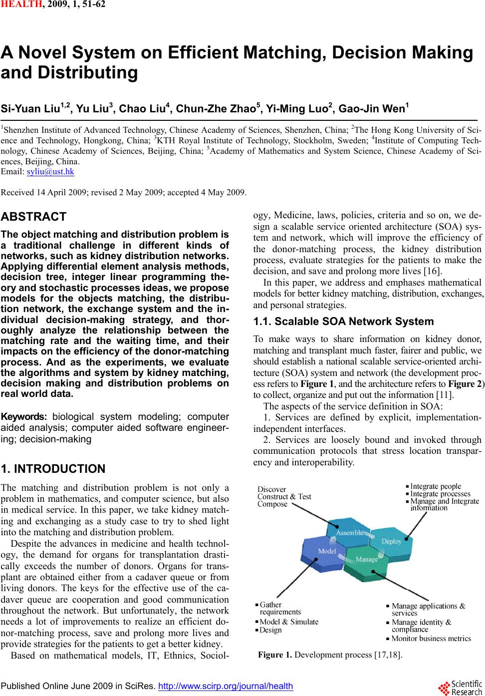HEALTH, 2009, 1, 51- 6 2
Published Online June 2009 in SciRes. http://www.scirp.org/journal/health
A Novel System on Efficient Matching, Decision Making
and Distributing
Si-Yuan Liu1,2, Yu Liu3, Chao Liu4, Chun-Zhe Zhao5, Yi - Ming Luo2, Gao-Jin Wen1
1Shenzhen Institute of Advanced Technology, Chinese Academy of Sciences, Shenzhen, China; 2The Hong Kong University of Sci-
ence and Technology, Hongkong, China; 3KTH Royal Institute of Technology, Stockholm, Sweden; 4Institute of Computing Tech-
nology, Chinese Academy of Sciences, Beijing, China; 5Academy of Mathematics and System Science, Chinese Academy of Sci-
ences, Beijing, China.
Received 14 April 2009; revised 2 May 2009; accepted 4 May 2009.
ABSTRACT
The object matching and distribution problem is
a traditional challenge in different kinds of
networks, such as kidney distribution networks.
Applying differential element analysis methods,
decision tree, integer linear programming the-
ory and stoc hastic proce sses ide as, we prop ose
models for the objects matching, the distribu-
tion network, the exchange system and the in-
dividual decision-making strategy, and thor-
oughly analyze the relationship between the
matching rate and the waiting time, and their
impacts on the efficiency of the donor-matching
process. And as the experiments, we evaluate
the algorithms and system by kidney matching,
decision making and distribution problems on
real world data.
Keywords: biological system modeling; computer
aided analysis; computer aided software engineer-
ing; decision-making
1. INTRODUCTION
The matching and distribution problem is not only a
problem in mathematics, and computer science, but also
in medical service. In this paper, we take kidney match-
ing and exchanging as a study case to try to shed light
into the matching and distribution problem.
Despite the advances in medicine and health technol-
ogy, the demand for organs for transplantation drasti-
cally exceeds the number of donors. Organs for trans-
plant are obtained either from a cadaver queue or from
living donors. The keys for the effective use of the ca-
daver queue are cooperation and good communication
throughout the network. But unfortunately, the network
needs a lot of improvements to realize an efficient do-
nor-matching process, save and prolong more lives and
provide strategies for the patients to get a better kidney.
Based on mathematical models, IT, Ethnics, Sociol-
ogy, Medicine, laws, policies, criteria and so on, we de-
sign a scalable service oriented architecture (SOA) sys-
tem and network, which will improve the efficiency of
the donor-matching process, the kidney distribution
process, evaluate strategies for the patients to make the
decision, and save and prolong more lives [16].
In this paper, we address and emphases mathematical
models for better kidney matching, distribution, exchanges,
and personal strategies.
1.1. Scalable SOA Network System
To make ways to share information on kidney donor,
matching and transplant much faster, fairer and public, we
should establish a national scalable service-oriented archi-
tecture (SOA) system and network (the development proc-
ess refers to Figur e 1 , and the architecture refers to Figur e 2)
to collect, organize and put out the information [11].
The aspects of the service definition in SOA:
1. Services are defined by explicit, implementation-
independent interfaces.
2. Services are loosely bound and invoked through
communication protocols that stress location transpar-
ency and interoperability.
Figure 1. Development process [17,18].

52 S. Y. Liu et al. / HEALTH 1 (2009) 51-62
SciRes Copyright © 2009 HEALTH
3. Services encapsulate reusable business function.
4. Services to good communication and more donors
for patients.
The service flow is as Figure 3 shows.
The system and network should also be designed to
base on web service, which provide an emerging set of
open-standard technologies that can be combined with
proven existing technologies to implement the concepts
and techniques of SOA.
Based on this kind of scheme, the transplant network
will come to a better status, that is, a better communica-
tion (which has been processed as services), a better ef-
ficiency, a better robustness and a better scalability [11],
especially making the communication and information
sharing aggregated services in a distributed heterogene-
ous network computing environment.
2. MATHEMATICAL MODELS FOR THE
TRANSPLANT NETWORK
2.1. Analysis of the Problem
The popular method nowadays is, to collect personal
information, evaluate the patients’ situation and give a
score, and then sort the patients by the score. When a
kidney appears and is available, the patient who has a
better matching rate, a higher priority and a higher score
will get it. This kind of scheme may come to an ap-
proximate best result, but after our extensive research, a
rigorous reasoning and innovative designs, we propose a
new program which will should save and prolong lives
as more as possible, and meanwhile cut the waiting time
for the patient as short as possible.
2.2. Assumptions
1) Everybody’ life obeys exponential distribution.
2) Malthus Model, Logistic Model and Regressive
Model are applied to forecast the population changing in
a short term (a year) [3].
3) The population can be divided into four classes:
a) Normal persons live without nephropathy, and with
two kidneys.
b) Normal persons live with only one kidney because
of a living donor.
Figure 2. Service oriented architecture [16,17,18].
Figure 3. SOA service flow [17].

S. Y. Liu et al. / HEALTH 1 (2009) 51-62 53
SciRes Copyright © 2009 HEALTH
c) The patients wait for cadaver and living donors, in-
cluding renal allograft dysfunctions after the first trans-
plant.
d) The patients are healthy now after transplant.
4) Because the demand for organs transplantation
drastically exceeds the number of donors, we assume,
physiologically, any kidney can get a match patient.
5) The transplant kidney’s life obeys exponential dis-
tribution.
6) The death rate of the patient in the waiting list is
higher than that of the population, but after transplant
operation, before the renal allograft dysfunctions occur,
the death rate of the patient is considered to be the same
as the normal, and from the study material, the death rate
of the operation is very low, maybe can be considered to
be 0.
2.3. Definitions and Key Terms
t is time, unit: year.
1
x
is the percentage of the patients waiting for do-
nors in the total population.
2
x
is the percentage of healthy patients after trans-
plant in the total population.
x3 is the percentage of available cadavers in the total
population at .
t
x4 is the percentage of healthy patients after living
donors transplant in the total population at .
t
()Nt is the total population at . t
() ()
ii
X
txNt, 1, 2,3, 4.i
a is the probability of serious kidney disease which
the patients need transplant in the population in a time
unit.
b is the death rate of the patients in the waiting list.
c is the rate of renal allograft dysfunction.
d is the average death rate in the total population.
h is the average number of kidneys from living donors
for a patient.
k is the productivity of the available cadavers in the
total population.
2.4. Design of the Model
The variation of at is )(
1tX ],[ ttt  ()
X
tt


()
X
t
Na (
bx
which should include the new increasing patients,
, from t to , the number of pa-
tients, , who have to wait for donors again be-
cause of renal allograft dysfunction and the variation,
, because of death, cadavers and
living donors.
tXX  )
21
tcx 
2
13
2tx th 
tt 
1
tx
So,
11
122 13 1
()-()
(- - )--2-
Xt DtXt
aNXXDtcXDtbx DtxDthx Dt


11
123
()()
()()2
X
ttXt abhXcaXX aN
t

 

Let 0

t, so
112
()()()2 3
X
tabhXcaX XaN 

while the variation of X2 mainly depends on renal al-
lograft dysfunction, the decrease from the normal death
and the increase from cadaver and living donors, so
2212
()()[()2]
3
X
ttXthXcdX Xt

  
And then,
21 2
()()2 3
X
thXcdX X 

The variation of available cadavers, X3, is a direct ra-
tio with the number of the healthy people at t, but, the
people who has made a living donor will only donate a
kidney after death, so
13 4
33 1434
1
()()( )
2
1
()
2
XttXtkNXXXtkXt
kNXX Xt

 
 
And then,
3124
1
() 2
X
tkXkX kXk 
N
4
.
Last but not least, we analyze the variation of X4.
Based on common sense, we would come to an analy-
sis that the living donor always chooses a direct trans-
plant to relatives or friends, so the variation of X
4 is
strongly relative to the variation of X1, meanwhile, these
donors with only one kidney left will live like a normal
person with the same death rate if they get the proper
care, so,
41
X
kX dX

.
Above all,
11
22
33
44
20
20 0
1
020
00
abh ca
XX
a
hcd
XX
d
N
XX dt kk k
XX
hd


 


 
 

 

 
 

 

 


 


 


k
(1)
The above equations describe our model system, and
if given an initial value, the system can forecast the
value of . Facts have proven that in
some years the forecast is quite accurate.
)()( 41 tXtX 
Coming to the goal of our network model design, it
should save and prolong more lives, and meanwhile
should cut the waiting time for the patient as short as
possible.
Let

54 S. Y. Liu et al. / HEALTH 1 (2009) 51-62
SciRes Copyright © 2009 HEALTH
0
0
[,]
[,]
f
f
J
the accumulative totalwaiting time intt
thenumber ofpatientswhogetthe properkidney intt

,
which is our index function, and apparently , and
the smaller J is, the better.
J0
Then we will calculate the expression of . J
'
0
110
()()()()
fff
t
NumeratorXtt tdtXtt t
t

0

0
)
f
0
110
t
=()()()(
ff
ttdXtXttt
t 

ff
11010
00
t=t t
=()()()()()
t=t t
f0 f
X
tt tXtdtXtt t 

f
10
0
t
=()
t
X
tdt
,
31
0
(2 )
f
t
DenominatorXhX dt
t

,
So,
1
0
313
00 0
1
0
1
min 22
f
ff f
f
tXdt
t
Numerator
Jtt t
Deno atorXdt hXdtXdt
tt t
h
tXdt
t
 



 

(2)
Then, we will solve the (1), and analyze the extremum
of with the result.
J
Let ,
TT
14
X=(XX ) 

……， =(a,0,k,0)
0
20
20
1
02
00
abh ca
hcd
Akk
h






 





k
d








.
Then the (1) becomes to be
X=AX+ N d
dt

 (3)
Because , let
, then
i
xN (i=1,2,3,4)
n
X123 x(x,x,x,=

4
x)
T
X= (xN)=N( x)+xN. ddd d
dt dtdtdt


So the (3) will be
0
Nx+xN=(A x+)N




 
0
x=A x+x
N
N
 




04
x=(A -IlnN)x+
d
dt




.
Let 04 IlnN
d
AA dt  , we notice that the percentage
of patients in the total population N(t) is very small, so in
the situation that 0f tt

is not large, such as 1
f
tt

,
we can apply the classic Malthusian Population Model to
describe N(t), and get


0
0
() ,
tt
Nt Ne
 
 so N
d
t
dln
const


, and then, 04
A
AI

 .
Based on the above process, the solution of the origi-
nal equation can be calculated by the following formula,
0
() 1
1
() At t xteC A





,
where 0
()
0
0
1()
!
At tn
n
eAt
n

n
t



, and is a
regular vector to be determined.
4
1RC
If given the initial condition
000
() ()
0
x
txXNt


,
We can determine
11
1000
()CxAXNt A



 



, so
0
() 1
0
() ()
At t
xtex AA1






, 0
[,]
f
ttt.
And with ()() ()
x
txtNt


, we can expediently calcu-
late the value of ()
X
t

.
Substituting into J with the expression of X

, it has
become the function of A. Considering a, b, c, d, h, k,
which have be defined, we can get that the death per-
centage of the patients in the waiting list, b, closely re-
late to the average length of waiting time. If we apply
Poisson distribution to describe the renal allograft dys-
function, so c approximately equals the reciprocal of the
average length of life after transplant, which is related to
requirements on the kidney medical matching before
distribution. The more strict requirements on the kidney
medical matching are, the longer the expected total
length of life of transplants. But and nearly are
effected by our kidney distribution policies because they
will just effect only very few patients’ life length, while
and reflect the psychological dynamics of the
people, which will not be directly changed by our dis-
tribution policies. So we should take and as con-
trollable variables, while search , , , from
the public data.
a
a
d
h
h k
b
d
c
k

S. Y. Liu et al. / HEALTH 1 (2009) 51-62 55
SciRes Copyright © 2009
We find that if c is given, J changes with b steadily,
A natural idea is to let and as small as possible.
In the actual operation, to decrease the average waiting
time, we have to loose the condition, while the average
waiting time will become longer, if we strict the re-
quirements on matching much more, so our goal is to get
the best combination of andc.
b
b
c
while when c increases, J decreases rapidly. So the bot-
tleneck of the current situation in America is c, that is,
the rate of renal allograft dysfunction. Based on these
analyses, we recommend that benefit the patients with
higher matching rate, and reduce the weight of waiting
time to let c as small as possible.
Because (1) is resolvable, and the form of the solution
ensures it is continuous derivative aboutt, so we substi-
tute
X

)
into it, and we can get the expressions of
(,
J
bc. In the actual work, this calculation is very com-
plex, but thanks to some powerful symbol computing
mathematical software, it will be quickly done.
Coming to the details, according to actual factors, you
should determine the domain of J(b,c), and then find the
nearest point (b0,c0) to axis c=0 in this area. If there are many
such points, you should take the smallest value of b as .
0
b
For example, considering
From the results, we come to the conclusion that
(,)
J
bc
(,
is continuous derivative about (b,c), and appar-
ently 0≤b≤1, 0≤c≤1. So it’s sure to get the minimum
of )
J
bc. Theoretically speaking, we can apply
2140
0.05 0.8
0.01 0.2
bc
c
b







0
0
J
b
J
c










based on the above rules, we should take 00
(, )bc

as data to assist guidance. You should adjust
next year’ distribution policy, when you find (b, c)
doesn’t accord last year’s statistical data.
(0.1,0.05)
0
bb

and
0
cc

will not appear because 21 40
bc
 . If ,
you should increase the weight of waiting time in the
next year’s evaluation policy; if , you should in-
crease the weight of matching rate.
0
bb
0
cc
to get the extremum from the solutions, and then screen
out. But in the actual work, we can apply numerical
methods to get the numerical solution, and even to ana-
lyze the trend of J by drawing the 3D imagines to guide
policies.
2.5. Testing and Result Analysis
After the analysis of data (2004-2005) in America, we
et the figure (Figur e 4) about J(b,c) as follows. g
Figure 4. J(b,c) situation analysis.
HEALTH

56 S. Y. Liu et al. / HEALTH 1 (2009) 51-62
SciRes Copyright © 2009 HEALTH
2.6. Conclusions and Solutions
When distributing kidneys, we are always tending to
hesitate on balancing waiting time and the matching rate.
Let’s take a case for example. A kidney matches a pa-
tient completely who just now entered the waiting list,
while it is barely compatible for a patient who has
waited for a year. Then the doctor will be puzzled how
to distribute this precious kidney. By using our model,
we could get the average latency time and the average
matching rate. If in the average waiting time, we should
consider the average matching rate firstly and distribute
the kidney to the patient with the best match, while out
of the average waiting time, we should distribute the
kidney to the patient with the longest waiting time.
The potential bottleneck is the contradiction between
matching rate and waiting time. We will evaluate the
latency risks during the waiting time in Ⅲ-A.
It is hard to say that the network divided into smaller
ones is good or not, because the situation varies from
state to state. In some areas the kidney resource is very
rare, while the situation is opposite in the other areas.
Establishing a large network could balance resources in
all fields. Of course, the patients must have an operation
immediately because the warranty for a cadaver kidney
is only 1-2 days [12]. For the reason of distance, it is
more appropriate to choose a donor in a nearer area.
Anyhow, it is feasible to substitute the data of the district
into our model and evaluate overall.
The ways to save and prolong more lives can be re-
flected by parameters b, c, h which are mentioned in our
model. In our distribution network, the index function is
0
0
[,]
[,]
f
f
J
theaccumulative totalwaitingtimeattt
the numberofpatientswho getthe properkidneyattt

We can change it to be J =the number of patients who
get the proper kidney. So we can decrease the restric-
tions to pursue the one and only target, saving and pro-
longing more lives, and the system will be more effec-
tive.
3. DISTRIBUTION DECISION TREE
3.1. Analysis of the Problem
As the number of organs for transplanting is restricted,
while a large number of patients need them, we have to
consider how to distribute these organs fairly, reasonably
and effectively.
The typical approach for distribute is linear matching
score (
1
n
ii
i
s
corew ab



), but we believe there are
several defects in this method.
1) Variables are difficult to normalize. For example,
0<age<100, commonly, as there are A, B, AB and O four
blood types. How to put them into a uniform and com-
parable range?
2) The weight for each variable is hard to confirm.
So we introduce the decision tree to get across this
morass. A decision tree is flow-chart-like tree structure,
where each internal node denotes a test on an attribute,
each branch represents an outcome of the test, and leaf
nodes represent classes or class distributions.
3.2. Attributes for Decision
We mainly consider these attributes while distributing:
a. Transplant centre effects
b. HLA match rate
c. Incompatibility rate
d. Patient renal disease
e. Waiting time
Each of them has characteristic itself. Based on these
characteristics, we classify them as follows.
Boolean Attribute: Transplant centre effects and Pa-
tient renal disease. Kidney transplanting should be oper-
ated as soon as possibly. If the distance between the
kidney and the patient is too far, it will be impossible to
make this operation. Based on this factor, patients should
be classified into two parts, incompatibility and com-
patibility. If the patient is suffering other disease, e.g.
AIDS or cancer, our advice is that they are not fit to dis-
tribute a kidney.
Continuous Attribute: HLA match rate and Incom-
patibility rate。Based on the number of match points, the
output results will be divided into many classes, such as
r>90%, 90%>r>60%, and r<60% or the top 10%,
20%~50%, and so on. Treatment will all depend on the
situation.
Consult Attribute: Waiting time. If a patient waits for
a kidney for a long time, he will have a priority.
The attributes we described are classic, and there are a
quantity of attributes worth to interpret, e.g. psychology,
age and so on. They can also be classified as we talked
about before and we will make further discussions in 3.3.
3.3. Description of Decision Tree
The basic algorithm for decision tree induction is a
greedy algorithm that constructs decision trees in a top-
down recursive divide-and-conquer manner. The basic
strategy is as follows.
The tree starts as a single node representing the in-
formation of patients which maybe in large scale and the
only kidney for distribute.
A branch is created for each known value of the test
attribute, and the patients are partitioned accordingly.
Finally, every patient are labelled by a leaf which rep-
resenting the match rate of the patient and the kidney, in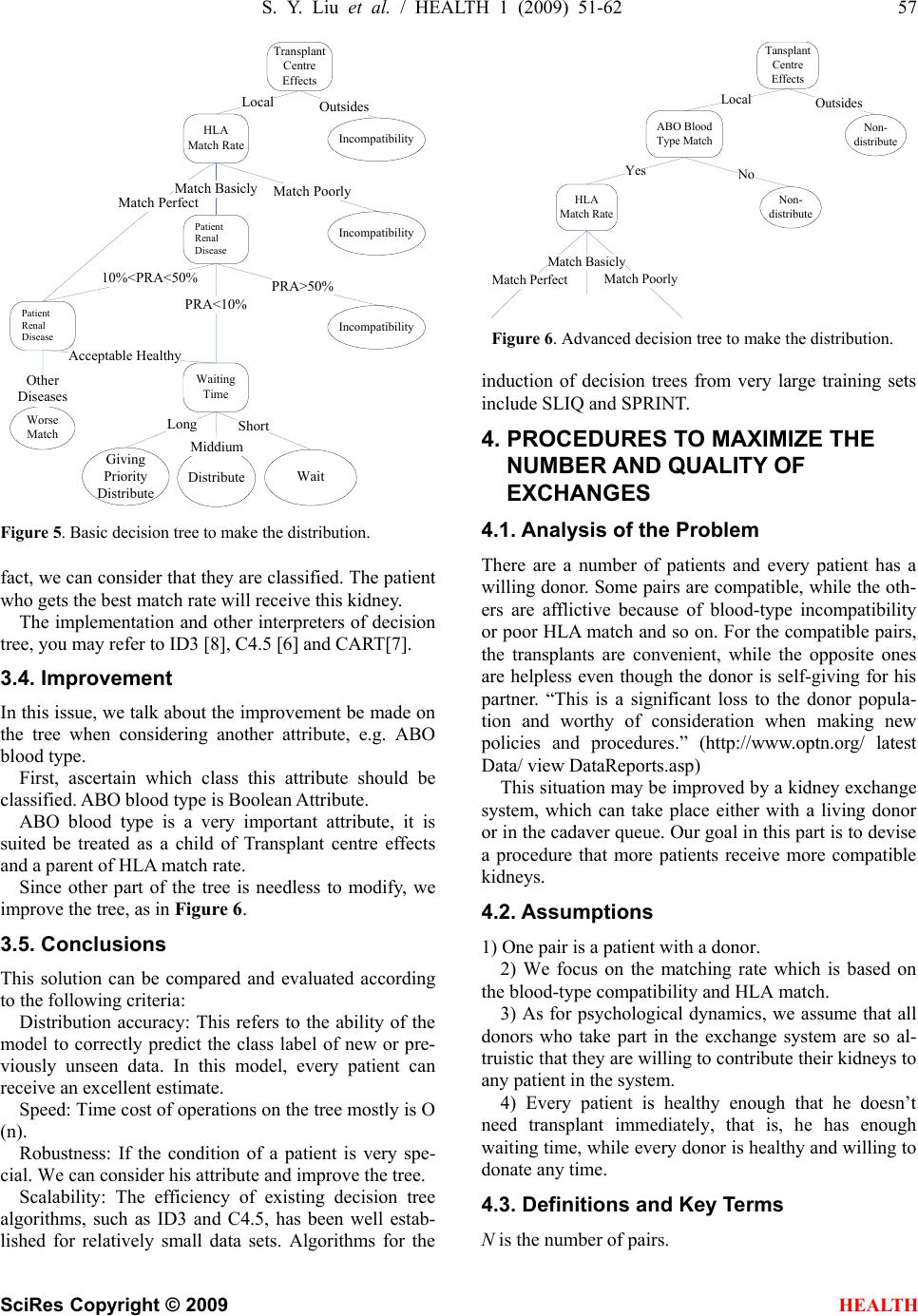

S. Y. Liu et al. / HEALTH 1 (2009) 51-62 57
SciRes Copyright © 2009 HEALTH
Transplant
Centre
Effects
Local
HLA
Match Rate
Patient
Renal
Disease
Match Perfect
Waiting
Time
Acceptable Healthy
Incompatibility
Outsides
Match Poorly
Patient
Renal
Disease
Match Basicly
Giving
Priority
Distri bute
Wait Distri but e
Long
Middium
Short
10%<PRA<50%
PRA<10%
Worse
Match
Other
Diseases
PRA>50%
Incompatibility
Incompatibility
Figure 5. Basic decision tree to make the distribution.
fact, we can consider that they are classified. The patient
who gets the best match rate will receive this kidney.
The implementation and other interpreters of decision
tree, you may refer to ID3 [8], C4.5 [6] and CART[7].
3.4. Improvement
In this issue, we talk about the improvement be made on
the tree when considering another attribute, e.g. ABO
blood type.
First, ascertain which class this attribute should be
classified. ABO blood type is Boolean Attribute.
ABO blood type is a very important attribute, it is
suited be treated as a child of Transplant centre effects
and a parent of HLA match rate.
Since other part of the tree is needless to modify, we
improve the tree, as in Figur e 6.
3.5. Conclusions
This solution can be compared and evaluated according
to the following criteria:
Distribution accuracy: This refers to the ability of the
model to correctly predict the class label of new or pre-
viously unseen data. In this model, every patient can
receive an excellent estimate.
Speed: Time cost of operations on the tree mostly is O
(n).
Robustness: If the condition of a patient is very spe-
cial. We can consider his attribute and improve the tree.
Scalability: The efficiency of existing decision tree
algorithms, such as ID3 and C4.5, has been well estab-
lished for relatively small data sets. Algorithms for the
Tansplant
Centre
Effects
Local
HLA
Match Rate
Match Perfect
Non-
distribute
Outsides
Match Poorly
Match Basicly
ABO Blood
Type Match
Yes
Non-
distribute
No
Figure 6. Advanced decision tree to make the distribution.
induction of decision trees from very large training sets
include SLIQ and SPRINT.
4. PROCEDURES TO MAXIMIZE THE
NUMBER AND QUALITY OF
EXCHANGES
4.1. Analysis of the Problem
There are a number of patients and every patient has a
willing donor. Some pairs are compatible, while the oth-
ers are afflictive because of blood-type incompatibility
or poor HLA match and so on. For the compatible pairs,
the transplants are convenient, while the opposite ones
are helpless even though the donor is self-giving for his
partner. “This is a significant loss to the donor popula-
tion and worthy of consideration when making new
policies and procedures.” (http://www.optn.org/ latest
Data/ view DataReports.asp)
This situation may be improved by a kidney exchange
system, which can take place either with a living donor
or in the cadaver queue. Our goal in this part is to devise
a procedure that more patients receive more compatible
kidneys.
4.2. Assumptions
1) One pair is a patient with a donor.
2) We focus on the matching rate which is based on
the blood-type compatibility and HLA match.
3) As for psychological dynamics, we assume that all
donors who take part in the exchange system are so al-
truistic that they are willing to contribute their kidneys to
any patient in the system.
4) Every patient is healthy enough that he doesn’t
need transplant immediately, that is, he has enough
waiting time, while every donor is healthy and willing to
donate any time.
4.3. Definitions and Key Terms
N is the number of pairs.

58 S. Y. Liu et al. / HEALTH 1 (2009) 51-62
SciRes Copyright © 2009 HEALTH
ij
x
where 1

1, 0xij

iN, 1jN, i, j 

Natural Number. If the patient in Pair i receives a kidney
from Pair j , , otherwise, .
1
ij
x0
ij
x
ij
r ，where 1iN, 1j[0%, 100 %]
ij
r

N, i,j

Natural Number. It is the match rate of the patient
from Pair i with the kidney from Pair j.
X
is the Matrix whose elements are ij
x
.
R is the Matrix whose elements are .
ij
r
4.4. Design of the Model
We build an Integer Programming model to determine
how to distribute all the kidneys to the appropriate pa-
tients. We have two kinds of best targets, which can be
applied in different situation:
1) The entity matching rate is maximal
2) The number of successful exchange pairs is maxi-
mal
First, Fill Matrix R using decision tree which we de-
scribed in session 3.
MODEL:
In Figure 7, the arrow shows a kidney is passed from
pa
ple, if we had not applied this exchange
sy
R=[63 0 68 0 0 93 0 0 77 62
82 0 0 0 0 0 89 70 79 76
0 0 0 0 0 86 0 0 89 0
0 0 77 0 58 68 67 100 0 94
57 0 0 0 0 0 97 0 78 0
0 75 0 0 74 0 78 89 93 100
0 61 0 89 0 67 0 0 0 0
60 0 0 0 0 72 78 0 0 61
90 0 67 63 0 83 0 65 0 60
60 0 0 0 66 0 0 75 0 0];
We solve the problem by Lingo 8.0, and the result is,
Objective value: w=822.0000
X( 1, 3) 1.000000 68.00000
X( 2,10) 1.000000 76.00000
X( 3, 9) 1.000000 89.00000
X( 4, 8) 1.000000 100.0000
X( 5, 7) 1.000000 97.00000
X( 6, 2) 1.000000 75.00000
X( 7, 4) 1.000000 89.00000
X( 8, 6) 1.000000 72.00000
X( 9, 1) 1.000000 90.00000
X( 10,5) 1.000000 66.00000
Objective function:
max result= (4)
T
RX
Constraints:
1
1
n
ik
i
X


; k=1, 2... n (5)
1
1
n
lj
j
X


; l=1, 2... n (6)
where (5) means one kidney can be only distributed to
one patient, while (6) means one patient only gets one
kidney.
This model is a classical Integer Programming which
can be solved by Lingo etc.
Based on the model, we establish our algorithm:
Step 1. Establish the database of all pairs, including
the blood types, HLA characters, and other personal
data like age, health situation etc.
Step 2. Fill the Matrix R through decision tree (as
we provide, or established by users themselves), refer-
ring to session 3.
Step 3. Solve the model, and gain a nice exchange
scheme.
4.5. Testing and Sensitivity Analysis
In order to illuminate how the procedure works, we
simulate a representative example.
We try our best to make sure that the data is random,
in order to make it universal. The Matrix R produced by
Matlab7.1 is as follows,
ir j to pair i.
In this exam
stem, only one pair can accomplish the transplant, that
is, Pair 1 whose matching rate is 63. However, through
taking part in the exchange system, all the pairs obtain
the gratifying kidney. This weight matrix can be consid-
ered to be consummate, but then, there are situations that
some pairs can not obtain appropriate kidneys even
though they donate kidneys to others. With the quit of
the satisfied pairs and entry of new pairs, this network is
Figure 7. An example of kidney exchange system.
dyna will mic, and in the next distribution, these patients

S. Y. Liu et al. / HEALTH 1 (2009) 51-62 59
SciRes Copyright © 2009 HEALTH
ger Programming, so the solution
who would like to exchange their
of the matching problem, maybe some of the
pa
5. STRATEGIES FOR THE PATIENT TO
5.1
nd awkward situa-
on that whether to take a
ba
5.2. Assumptions and Definitions
have the priority to get donor or cadaver kidneys.
4.6. Justification
Because we apply Inte
maybe is the best, and we take the pairs in the system
fairly, so the matching process and result is meaningful
for the current exchange system.
4.7. Conclusions
In this model, all pairs
organs register at first, and then the system collects the
information which is useful in the organ matching. Fol-
lowing the procedure that is proposed in 4.4, we can get
the data that how many more annual transplants will
generate.
Because
tients can’t get kidneys even though they have provided
kidneys for others. But to advocate donors, as compensa-
tion these people will rank a higher priority in the waiting
list, while patients in the current waiting list have a willing
but incompatible donor will benefit for this exchange sys-
tem, and you will get the number of the more annual trans-
plants through the procedure we proposed.
MAKE A BETTER DECISION
. Analysis of the Problem
A patient maybe always face a hard a
tion and need a strategy to decide whether to take an
offered kidney, wait for a better match from the cadaver
queue or to participate in a kidney exchange. We pro-
pose a strategy considering the risks, alternatives, and
probabilities to help patients to make a better decision
and come to a better result.
When facing the situati
rely compatible kidney, the patient should consider
and evaluate the risk of waiting, the effect of transplant,
and the financial factors to make a decision. After study
a mount of relative materials, we find out that there are
different exchange modes in different countries. To be
clear, we take a popular mode as an example to study
and discuss, which is, once a patient decides to partici-
pate in a kidney exchange, and put out an offer, then he
will get a very authorized promise that he will get a bet-
ter matching kidney in a given certain time.

is the left life length of the patient.

is the interval length between two offers(last offer
he gave up, and this offer he is waiting for) for the pa-
tient.

is the normal life time length of the transplanted
kidney.

,

, and

all obey exponential distribution, and
their parameters are expectable, and

,

, and

are
statistical independent. The parameters of

,


, are
relative to matching rate, the health conditioofe pa-
tients and the donors and the donors kidneys. Let
n th


is
directly proportional to the matching rate, that is, after a
patient took a cadaver kidney, 1(0) r




, where
(0,1]r

is the matching rate. (0)


is a const deter-
the condition of the patient. Under the same
condition, the living donors let
mdine by
1(0)
1r
2




.
Our goal is to design the bes tht strategy fore patient
w
eir in
y the distribution policies in the
the
hen he faces the situation that whether he should take
the offer. So we don’t consider the death caused by other
factors other than nephropathy. For a certain patient, r,
a random variable, obeys uniform distribution on 0 [,1r.
(Other distributions can be solved by applying th-
verse functions, which refer to Angel R. Martinez and
Wendy L. Martinez).
0
r is determined b
]
network.(e.g. some network only distributes kidney to
the patient with the matching rate higher than 50%, so
0
r=0.6). Because the probability of the death caused by
transplant operating is very small and minimally
different for different patients, so we assume the patients
will not die on the operating table.
5.3. Design of the Model
Let { }Lptransplant successE


, because during the
in
th
use the offers whose matching
ra
, and-
ch
waiti ace the nephropathy
death risk, and after successful transplant, before the
renal allograft dysfunctions, the patients will enjoy the
normal life, so L characterizes the expectation of the
patient after makg a decision, which is our index func-
tion.
Our goal is to propose a strategy for the patients to let
L
ng time, the patients will f
maximum. And the alternative programs are:
Strategy 1. Take the first offer without hesitation, and
e matching rate is f r.
Strategy 2. Always ref
te is lower than e r, until get the kidney with e rr.
Strategy 3. Participate in a kidney exchange ex
ange the barely compatible kidney with our needy
patients.
The details of the model are as follows.
Take the first offer without hesitation.
Based on assumption 5 (Ⅱ,B),
{ }1Psuccessful transplant

60 S. Y. Liu et al. / HEALTH 1 (2009) 51-62
SciRes Copyright © 2009 HEALTH
So,
1
)
[1]
Wait for a match fradaver queue.
1(0)
11( f
E r

 

L
e
rr om the c
{ }successful ant
{ }
P transpl
Pthe cadaverkidneyarrives before the patientdies
1
{ }
*{ }
n
e
th
th
Pthe nofferarrives before the patientdies
Pthe firsttime thatthe noffersatisfies rr





1
0
100
1
{}*()
11
n
ee
n
n
rr r
Prr 






.
Because n

is independent identical distribution
with

.

and

are statistical independent, so
{ }Pscessfultransplant
0
{}
xy
yx
uc
P
ee dxdy









00 {}
x
dxEXPxy dy
 
 


 






.
So,
2
1
(0) 1
*
()
(1)()
2( )
e
LE
r





















Participate in a kidney exchange.
fer obeys truncated
ex
The waiting time for the next of
ponential distribution, and let T the longest time to get
the promised kidney, so
() {FtP
0
}
1
{} 0
00
t
t
if tT
EXPtdt if tT
if t













 



And then,
}{Psuccessf }{ul transplantP


0
()
x
yx
edxdFy







0(() (0))
x
eFxFd




 

x
x
dx
dx
x
00
()
Tx
xy
T
eedydxe
 
 

 




0(1 )
Txx x
T
eedxe
 
 



 


()
0
1Tx ed







()
1(1
T
e

 




 
)
()T
e



 

 


 .
So,
3
1
{ }*
{ }
LPsuccessful transplantE
Psuccessful transplant






(0)1
1
{ }2(1)(
2
f
Psuccessful transplantr

 )


() (0) 1
(1)[]( )
T
f
rea

 

 
 
 
 
 
 .
5.4. Testing and Sensitivity Analysis
If we want to compare and , just need to know
the values of
1
L
,
3
L
,,
f
rT



 , and are all already
known. Because
,
f
rT

and

all obey exponential dis-
tribution, so11
,EE






 , and then
1
(),E




1
()E




.
Because E

is the expected left life length of the pa-
tient without transplant, while E

is the average wait-
ing time length for the next kidney, which can all be
estimated from the public data.
For example, in a country, the average lasting time for
a patient without transplant is 10 years, and the average
waiting time for a patient to get transplant is 5 years, so
. 0.1, 0.2

 
If 60%, 5
f
rT

, then
(0) 1(0) 1(0) 1
1
0.2 2
60%()()0.4( )
0.1 0.25
L
 
 


 

(0)1
3
(0) 1
1.5
0.2 0.1
(160%) [] ()
0.1 0.20.1 0.2
1.1857( )


Le





 


So in this situation, the patient should take part in ex-

S. Y. Liu et al. / HEALTH 1 (2009) 51-62 61
SciRes Copyright © 2009 HEALTH
change.
From the above process, we can come to the conclu-
sion that, the larger


,
f
r and T are, the smaller


is, and then the strategy should be taking the offer right
now; the smaller


,
f
r and T are, the larger


is,
then the strategy should be taking part in exchange and
waiting for a better kidney.
5.5. Strength and Weakness
Based on our assumptions, the distribution of any event
a patient may face is clear, that is, we can expediently
calculate the expected values, variances and so on. So
we have conditions to design different index functions.
We tried the following index functions,
{
| ,
}
i
th
K
Etheleft lifetimeofthepatients
who are makingthe decision
at most transplant kidneys twotimes
choose the istrategy

1, 2, 3i
After analyze the decision tree, we can get the expres-
sions of K1, 2
K
, and 3
K
, and easily solve them. But
finally we discard it, because of the following analysis.
The average life length of transplant kidneys is almost
10 years, we can not forecast what will happen in this 10
year, such as the death caused by other factors, and the
man-made kidney technology progress rapidly, so it’s
not meaningful to make a 20-years forecast ( transplant
kidneys two times).
{
| }
i
th
CEthe expense before
the firsttransplant
choosethe istrategy

1,2, 3i,
Because C increases with the expected waiting time
for the first transplant, and for the same person, the pro-
portion coefficient is the same, so we can let it 1.
So
10C;
2
00
{min{,}|2}
() ()() ()
xy yx
CE
x
dFx dFyydFx dFy
 

 



'
'''
11


'
2







 



,
where '
0
1
1
ey
r
r




, so
0
2
0
2(1 )
(1 )(1 )
e
r
Crr



 .
3
00
{min{,}| 3}
() ()() ()
xy yx
CE
x
dFx dFyydFx dFy
 

 



000
() ()
Ty x
x
T
dF yxedxdFydF y






 

C can be applied as the index to evaluate strategies,
which is the smaller the better.
5.6. Conclusions
By far we have established the model with all the ex-
pressions and equations for the strategy. After the sys-
tem calculate the three results, , and , the
patient just need to compare and choose the maximum.
1
L2 L3 L
Note: Considering0 01
fe
rrr ,


32
0LL
, and T, we can get .
(0)
,,,

 
00
So in the actual strategy, the patients just need to
choose between “take it right now” and “take part in
exchange”. It is apparent and easy to explain that, re-
ceiving an offer is an opportunity, but in strategy 2, the
patient gives it up just because it’s not satisfied, while in
strategy 3, this opportunity is used fully and becomes an
advantage.
6. DISCUSSIONS AND PROSPECTS
In the donor kidney distribution, whether an individ-
ual or entity, the matching rate is very important and
we should try our best to match the kidneys. While
the waiting time is not necessarily the most important
factor, so the patient should participate in kidney ex-
change, rather than get a rarely matching kidney.
Because in some acceptable wait time, he has a very
high probability of getting a good matching rate kid-
ney.
In the waiting list, the patient with the payback who
has given up a kidney should get the highest priority.
The illness condition of the patient is another impor-
tant factor to determine the order of the patient in the
waiting list. When the condition is quite serious, so the
more time the patient waits, the greater the probability of
his death is. For this kind of patients, it is necessary to
loose the matching requirements and give them priority
to get kidneys. And our system can achieve the ap-
proximate global optimal solution.
Our model can also be applied to online products dis-
tribution, the satisfaction rate of the customs is just like
the matching rate in our model.
With the progress of the technology and society,
maybe we should pay close attention to organ clone

62 S. Y. Liu et al. / HEALTH 1 (2009) 51-62
SciRes Copyright © 2009
[10] C. L. Li and L. Y. Li (2003) Apply agent to build service
management [J], Journal of Network and Computer Ap-
plications, 26, 323-340.
technology, organ sale legalization and the increasing
single kidney crowd.
[11] M. Keen, A. Acharya, S. Bishop, A. Hopkins, S. Mil-
inski, C. Nott, R. Robinson, J. Adams, and P. Ver-
schueren, (2005) Patterns: Implementing an SOA using
an enterprise service bus.
7. ACKNOWLEDGEMENT
The paper is supportted by 2008-China Shenzhen Inovation Technol-
ogy Program (SY200806300211A). [12] OPTN, SRTR. (2005) The U. S. organ procurement and
transplantation network and the scientific registry of
transplant recipients, 2005 OPTN / SRTR Annual Re-
port.
REFERENCES
[1] A. R. Martinez and W. L. Martinez, Computational sta-
tistics handbook with MATLAB, CHAPMAN & HALL/
CRC.
[13] S. Oliver, V. B. Prasad, D. Nigel, et a1., (2003) Leveraging
the grid to provide a global platform for ubiquitous com-
puting research, Technica1 Report Lancaster University,
CSEG/2/03 [EB/OL].
[2] A. Schrijver, (1986) Theory of linear and integer pro-
gramming, Wiley-Interscience Series in Discrete
Mathematics. [14] Shafer, Agrawal, Mehta, (1996) SPRINT: A scalable paral-
lel classifier for data mining [C], Proceedings of the 22nd
International Conference on Very Large Data Bases Mum-
bai, India.
[3] B. B. Dunaev, (1986) Statistical model of change in
population numbers, Cybernetics and Systems Analysis,
22(4), July. [15] H. Yamada and T. Kasvand, (1986) DP matching method
for recognition of occluded, reflective and transparent
objects with unconstrained background and illumination,
in Proc. 8th Int. Conf. Pattern Recog., Paris, 95-98.
[4] E. Newcomer and G. Lomow, (2004) Understanding
SOA with web services (independent technology guides),
Addison-Wesley Professional.
[5] Y. Hao, Y. H. Ding, G. H. Wen, (2001) SOAP protocol
and its application [J], Computer Engineering, 27(6),
128-130.
[16] E. Newcomer and G. Lomow, (2005) Understanding
SOA with web services, Addison Wesley, ISBN 0-321-
18086-0.
[6] J. R. Quinlan, (1993) C4.5: Programs for machine learn-
ing, Morgan Kaufmann Publishers Inc., March. [17] M. Bell, (2008) Introduction to service-oriented model-
ing, service-oriented modeling: service analysis, design,
and architecture, Wiley & Sons, 3, ISBN 978-0-470-
14111-3.
[7] L. Breiman, J. H. Friedman, R. A. Olshen, and C. J.
Stone (1984), Classification and regression trees,
Wadsworth International Group, Belmont, California.
[8] J. R. Quinlan, (1986) Induction of decision trees, Ma-
chine Learning, (1), 81-106. [18] T. Erl, (2005) Service-oriented architecture: Concepts,
technology, and design, Upper Saddle River: Prentice
Hall PTR, ISBN 0-13-185858-0.
[9] M. Mehta, R. Agrawal, and J. Rissanen (1996) SLIQ: A
fast scalable classifier for data mining, Extending Data-
base Technology.
HEALTH