 Journal of Applied Mathematics and Physics, 2014, 2, 235-251 Published Online April 2014 in SciRes. http://www.scirp.org/journal/jamp http://dx.doi.org/10.4236/jamp.2014.25029 How to cite this paper: Perkovac, M. (2014) Maxwell’s Equations as the Basis for Model of Atoms. Journal of Applied Mathematics and Physics, 2, 235-251. h ttp://dx.doi.org/10.4236/jamp .2014. 25029 Maxwell’s Equations as the Basis for Model of Atoms Milan Perkovac The First Technical School TESLA, Klaiceva 7, Zagreb, Croatia Email: milan@drivesc.co m Received February 2014 Abstract A century ago the classical physics couldn’t explain many atomic physical phenomena. Now the situation has changed. It’s because within the framework of classical physics with the help of Maxwell’s equations we can derive Schrödinger’s equation, which is the foundation of quantum physics. The equations for energy, momentum, frequency and wavelength of the electromagnetic wave in the atom are derived using the model of atom by analogy with the transmission line. The action constant A0 = (μ0/ε0)1/2s02e2 is a key term in the above mentioned equations. Besides the other well-known constants, the only unknown constant in the last expression is a structural con- stant of the atom s0. We have found that the value of this constant is 8.277 56 and that it shows up as a link between macroscopic and atomic world. After calculating this constant we get the theory of atoms based on Maxwell’s and Lorentz equations only. This theory does not require knowledge of Planck’s constant h, which is replaced with theoretically derived action constant A0, while the replacement for the fine structure constant α−1 is theoretically derived expression 2s02 = 137.036. So, the structural constant s0 replaces both constants h and α. This paper also defines the statio- nary states of atoms and shows that the maximal atomic number is equal to Zmax = 137. The pre- sented model of the atoms covers three of the four fundamental interactions, namely the electro- magnetic, weak and strong interactions. Keywords Action Constant, Fine Structure Constant, Lecher’s Line, Maxwell’s Equations, New Elements, Phase Velocity, Planck’s Constant, Stability of Atoms, Standing Waves, Stationary States, Synchronized States, System of the Elements, Structural Coefficient, Structural Constant, Transmission Line, Undiscovered Elements 1. Introduction During the whole of twentieth century physics has mostly been searching for answers to fundamental questions of matter, primarily the relationship between waves and particles. Discussions on this have not yet been completed. It is believed that natural laws are exactly the same in the macro and micro world. But this general approach to the macroscopic and microscopic scale seemed questionable in the case of Max- well’s equations. In fact, Maxwell’s equations have reached excellent results in the macroscopic scale. Their ap-  M. Perkovac plication in the microscopic scale at first glances seemed disappointing. Actually, Maxwell’s equations previously couldn’t explain stability of atoms (with respect to the radiation energy of those particles which are moving with acceleration), the periodic table of elements, the chemical bond, the discrete excitation energies of atoms and their energetic state, the ionization of atoms, the spectra, including its fine structure and transition rules, experimental evidence about X-ray spectra and the behavior of atoms in electric and magnetic fields, as well as the properties of matter in solid state. That was the reason why classical physics failed when applied to the atomic area, i.e., to the area of nanometers or below. Thus entire physics divided into two branches, namely, traditional, classical physics and new, quantum physics. Despite the uncertain physical meaning of the wave function at the famous Schrödinger’s equation, ∇2ψ + 8π2m(W-U)ψ/h2 = 0, the equation has played an important role in the development of quantum physics. The wave function ψ(x,y,z) = ψ(r) is the solution of the Schrödinger equation, i.e., it is a mathematical expression involving coordinates (x,y,z) of a particle in space, or expressed as a vector r = xi + yj + zk, where i, j and k are unit vectors in the Cartesian coordinates (all vectors below are bold cursive letters). If we solved the Schrödinger equation for a particle in a given system then, depending on the boundary condition, the solution is a set of allowed wave functions of the particle, each corresponding to an allowed energy level. The usual interpretation of the wave function ψ is that the square of its absolute value, i.e. |ψ|2, at a given point is proportional to the probability of finding the particle in a small element of volume, dxdydz, at that point. All of this was obtained without the use of Maxwell’s equations, in the early twentieth century. However, after the explanation of radiation [1-4], Maxwell’s equations can now contribute to modern physics much more than before. From Maxwell’s equations we derive Schrödinger’s equation, which is the basis of quantum physics. New findings may lead to a new interpretation of Schrödinger’s equation. The meaning of physical quantities in Maxwell’s equations is completely clear. Therefore, the meanings of the wave functions of these equations, which are derived from Maxwell’s equations, are also completely clear. This paper describes many atomic phenomena with the help of classical physics and shows how Schrödin- ger’s equation is obtained by using Maxwell’s equations. In this way, the above-mentioned disadvantages of classical physics can now be explained in the framework of classical physics. 2. Derivation of Wave Equations 2.1. Wave Equation in the Atom Maxwell’s equations are the four differential equations describing the space and time, i.e., (r, t), dependence of the electromagnetic field [5-10]: Gauss’s law for electric flux (electric flux begins and ends on charge or at infinity); (1a) Gauss’s law for magnetism (where magnetic field lines have no beginning or end); (1b) Faraday’s law of electromagnetic induction; a changing B produce E; , (1c) Ampère’s circuital law (with Maxwell’s correction); H is produced by current J and by changing D; (,) (,) (,)t tt t ∂ ×=+ ∂ D Hr Jr r ∇ (1d) where D is electric displacement, E is electric field strength, B is magnetic flux density, H is the magnetic field strength, ρ is volume charge density, and J is electric current density. Differential Hamilton’s operator is called “del” or “nabla” operator is a symbolically vector. There are a total of 16 variables in (1a)-(1d) (the 15 components of five vectors E, D, B, H, J, and the scalar ρ). If the source densities ρ and J are given (four known variables) there still remain 12 unknown variables. There are, however, eight equations; one from (1a), one from (1b), and three for components in (1c) and (1d) each. Obvi- ously, to make this system determinate we need additional relations. 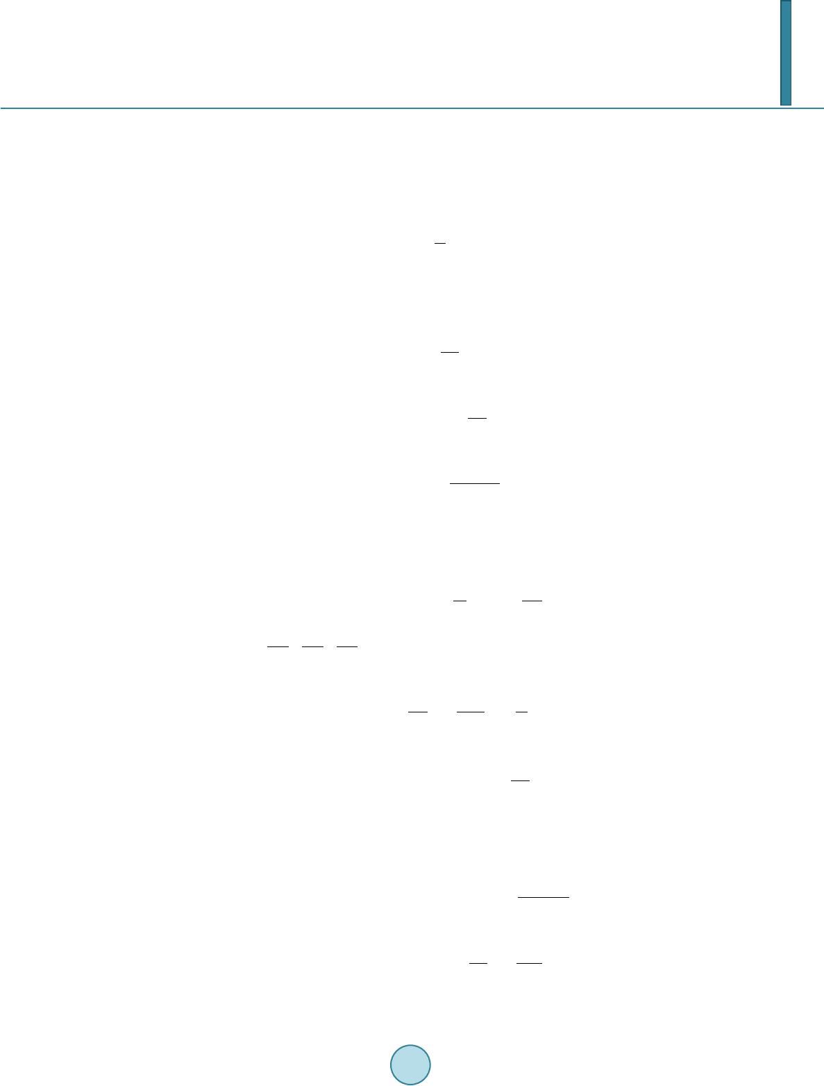 M. Perkovac For a completely linear medium there are constitutive relations describing the properties of the media in which the fields exist: D = εE, B = µH, J = gE, where ε is permittivity, ε = εrε0, where εr is relative permittivity, ε0 is permittivity of free space, µ is permeability, µ=µrµ0, where µr is relative permeability, µ0 is permeability of free space, and g is the conductivity of the media. Hence [without writing (r, t) which is implied] Maxwell equa- tions become: Gauss’s law for electric flux; , (2a) Gauss’s law for magnetism; , (2b) Faraday’s law; , (2c) Ampère’s law; . (2d) 1) Let’s take curl on Faraday’s law, i.e., on Equation (2c): . (3) On the other hand, for each vector E the following is true: , (4) and the substitution in Equation (3) Ampere’s law from Equation (2d) gives: 2 () tt µ εµ ∂∂ −−+ ∂∂ EE J E =∇ ∇⋅∇ , (5) where del-squared is an operator called the Laplacian. Now in Equation (5) add Gauss’s law for electric flux, i.e., Equation (2a), and J = gE: 2 220gtt ρ µ εµε ∂∂ −− −= ∂∂ EE E∇∇ . (6) 2) Let’s take curl on Ampère’s law, i.e., on Equation (2d): () () t µ εµ ∂ ××=×+ ∂ E BJ∇∇ ∇ . (7) On the other hand, for each vector B the following is true: . (8) Using J = gE here gives: 2() ( )()+gt µ εµ ∂× −× ∂ E BB E=∇ ∇ ∇⋅∇∇ . (9) Including Faraday’s law from Equation (2c) into Equation (9) we get: 2 22 () gtt µ εµ ∂∂ − −− ∂∂ BB BB=∇ ∇⋅∇ . (10) Using Equations (2b), i.e., , and B = µH, and after sharing with µ, we get from Equation (10) we 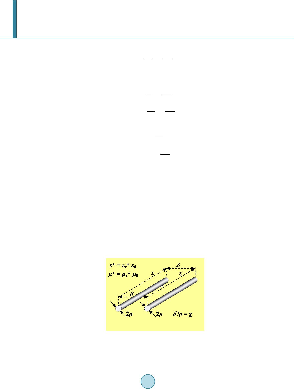 M. Perkovac get: . (11) Equations (6) and (11) are the required wave equations. These two vector equations constitute six component equations with seven unknowns (Ex, Ey, Ez, Hx, Hy, Hz, ρ). The system becomes determined if viewed without charge, i.e., when ρ = 0. So we get from Equations (6) and (11): , (12) . (13) In free space, i.e., in vacuum, what is also the inside of atoms is g = 0, so the Equations (12) and (13) become: , (14) , (15) where, [9], , (16) and (1 7 ) is phase velocity of electromagnetic wave, where λ is the wavelength and ν is the frequency of the wave. When processing the previous wave equations, there were no requirements that would exclude atoms. So you should take that Equations (14) and (15) are valid within the atom. 2.2. Wave Equation on Lecher’s Line Maxwell’s equations and Kirchhoff’s laws, [11,12], give the differential equation of voltage and current on Lecher’s line (i.e., on parallel-wire transmission line, consisting of a pair of identic ideal conductive nonmag- netic parallel wires of radius ρ, separated by δ, where the ratio δ/ρ = χ), Figure 1: Figure 1. Lecher’s line (section); twin-lead transmis- sion line consisting of pair of ideal conductive non- magnetic wires of diameter 2ρ, separated by δ situated in space with permittivity ε* = εr* ε0 and permeability μ* = μr* μ0. 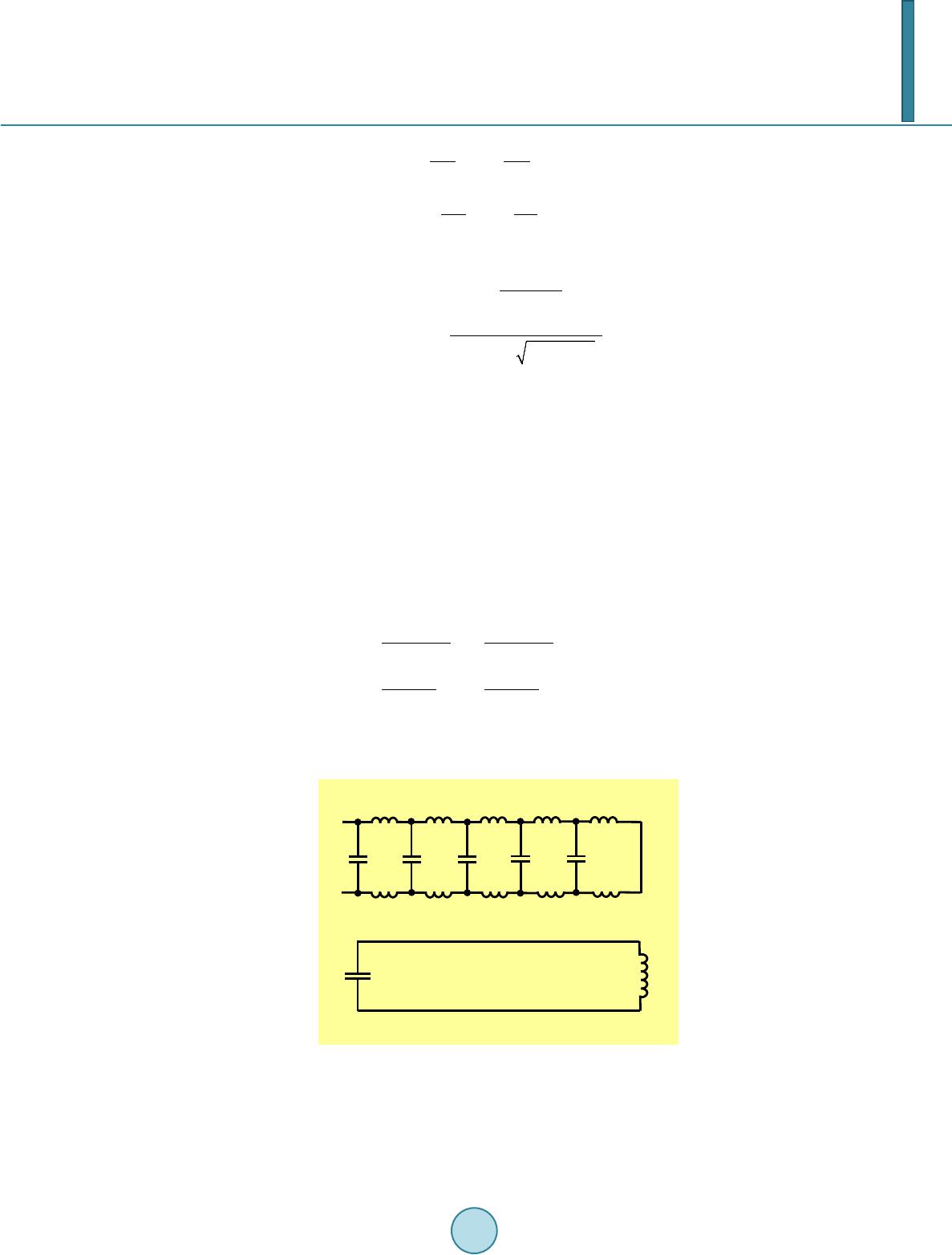 M. Perkovac , (18) , (19) where L’ is inductance of Lecher’s line per unit length, and C’ is its capacitance per unit length [7,13], Figure 2: , (20) () 2 r0 'ln/2+(/2)1 C π εε χχ ∗ =− , (21) where εr* is relative permittivity and µr* is relative permeability in the space of Lecher’s line (ε* = εr*ε0, µ* = µr*µ0). 3. Analogy between the Atom and Transmission Line For electromagnetic wave in an atom [Equations (14) and (15)], and for the wave of voltage and current on the transmission line (voltage/current wave) [Equations (18) and (19)], the same differential equations actually ap- ply [14]. Physical phenomena, described using the same differential equations, behave the same. This basically means that a study of voltages and currents at the Lecher’s line may conclude the behavior of electromagnetic waves in an atom. In this case, the voltage u(z,t) on the line will represent the electric field Ex(z,t) of the elec- tromagnetic wave, while the current line i(z,t) to represent Hy(z,t) the magnetic field of the electromagnetic wave [14]. Take Hy(z,t) and i(z,t): 22 yy 22 22 22 (,)(,) 0, ' '0. (,) (,) H ztH zt zt ii LC zt zt zt εµ ∂∂ −= ∂∂ ∂∂ −= ∂∂ (22) Now apply same relations to the electric field Ex(z,t) of the electromagnetic wave and voltage u(z,t) the Lech- er’s line, i.e., Figure 2. Lecher’s line is presented by an infinite number of extremely small uniformly distributed capacitors, with capa- citance C'dz, and inductors, with inductance L'dz, (a); all these capacitances are collected at the open end of the line, denoted by C*, and inductances on its short-circuited end, denoted by L*, resulting in a LC circuit, (b).  M. Perkovac 22 xx 22 22 22 (,)(,) 0, (,) (,) ' '0. E ztE zt zt uzt uzt LC zt εµ ∂∂ −= ∂∂ ∂∂ −= ∂∂ (23) Below we determine the parameters of Lecher’s line, along which we will equate the behavior of electromag- netic waves in the atom and the voltage/current waves on Lecher’s line by phase velocities, energies, frequen- cies and wavelengths. 3.1. Phase Relations of Waves in the Atom and Voltage/Current Waves on the Lecher’s Line Electromagnetic waves in the atom and the voltage/current wave on Lecher’s line will behave equally in phase velocity if the phase velocity of the electromagnetic wave in an atom uem is equal to the phase velocity of vol- tage/current wave on Lecher’s line, uem = uvc*, i.e., in accordance with the Equations (22) and (23) (24) From Equations (16), (17), (20) and (21) we get: [] r 00 0r rr 02 2 1 ln 4 () ln 1 24 =F χεµεµ εµεµ εµχ χχ ∗∗ ∗∗ + = +− , (25) em vc r0 0r rr 1()() , Fc F uu χχ εµ εεµµ εµ ∗∗ ∗ ∗∗ == == (26) where c = (ε0μ0)−2 is speed of light in vacuum and in accordance with Equations (25) and (26) is () 2 ln24 1 () ln1 4 F χχ χχ +− =+ , (27) em r emr0 0r r () u Fu c εµ χ εµεµ ∗ ∗ ∗ ∗ = = , (28) provided that = . Solving next two equations with two unknowns, i.e., μ*/ε* = μ0/ε0 and F(χ) = (ε*μ*)1/2uem, we obtain: 0 00 em 0 00 em em em 00 r r rr () , () , 1 ()( ). F u F u Fc F uu εχ ε εεµ µχ µ µµε χ εµ χ εµ ∗∗ ∗∗ ∗∗ = = = = = == (29) 3.2. The Energy of the Electromagnetic Wave in the Atom and the Energy of the Voltage/Current Waves on Lecher’s Line The total electromagnetic energy density, [6], is (E•D + B•H)/2. Electromagnetic energy, i.e., the energy of an electromagnetic wave in an atom Eem is obtained by integrating this expression at a time throughout the entire space of the wave: ( ) em 1ddd 2 E xyz= ⋅+⋅ ∫ ED BH . (30)  M. Perkovac On the other hand electromagnetic energy in the atom is obtained also by using the energy balance in the atom. From the balance of forces in the atom follows [15]: 2 2 2 22 2 1 || || ; 44 1 m qQqQ r r mc r β ε εβ β − = = ππ − v , (31) where r is the radius of the circular orbit of the electron, q is the charge of the electron (q = –e), e is elementary charge, Q is the charge of the nucleus (Q = Ze), Z is atomic number (which theoretically is not in integer do- main), m is the electron rest mass, c=1 /( μ0ε0)1/2 is the speed of light in vacuum, β = v /c, where v is the velocity of the electron, ε = εrε0, as stated above is permittivity, εr is relative permittivity, ε0 is permittivity of free space, μ=μrμ0, as stated above is permeability, μr is relative permeability, μ0 is permeability of free space, the transverse mass of the electron is m/(1 – β2)1/2, [16]. Increase of transverse mass of the electron is ∆ m = m/(1 – β2)1/2 – m. The kinetic energy of the electron, [15], is K = ∆ mc2, Figure 3: (3 2 ) Using Equation (31) and noting that an electron holds an opposite charge to the nucleus, the potential energy of electron, [12,15], is: . (33) The total mechanical energy of an electron W, [15], is the sum of its kinetic and potential energies: , (34) and according to the law of conservation of energy is equal to the negative emitted electromagnetic energy, Eem, 22 em 11EWmceV β =−=−−= , (35) where V is the potential difference through which the electron passes to get an equal energy as electromagnetic energy. W=K+U= -mc 2 [1-(1-β 2 ) 1/2 ]= -E em = - eV Figure 3. Energy relations in an atom (these relationships are valid for both classical and quantum physics; please note that the normalized quantities are marked with *). Radius of the circular orbit of the electron *r = r/[10|qQ|/(4πεmc2)], kinetic energy of the electron *K = K/(mc2), potential energy of the electron *U = U/(mc2), total mechanical energy of the elec- tron *W = *K + *U, electromagnetic energy of the atom *Eem = –*W = *eV; all versus normalized velocity of the electron β = v/c.  M. Perkovac Out of the Equation (35), Eem = mc2[1 – (1 – β2)1/2], comes (1 – β2)1/2 = 1 – Eem/mc2 and β2 = 2Eem(1 – Eem/2mc2)/mc2, so the radius r in Equation (31) through arranging leads to: 2 em 2 emem 1/ || 1 /2 E mc qQ rEE mc ε − =8π − , (36) or 22 em em em 22 em em 1/ 1/ 1| |1|| . 24 2 1 /21 /2 E mcE mc qQ EU rE mcE mc ε −− = = π−− (37) On the other hand Lecher’s line can be shown as the inductive-capacitive network (so-called LC network), which finally makes the oscillatory circuit (LC circuit), Figure 2, [11]. The natural frequency ν* of LC circuit is [15]: , (38) where C* is the sum of all small capacitances of the LC network on the open end of the network, and L* is sum of all small inductances of the LC network on the short-circuited of the network [11]. To realize the analogy between atoms and transmission lines according to the model presented in [14], electromagnetic energy in the atom Eem can be described as the electromagnetic energy of LC circuit, i.e., , (39) where Θ is maximal charge on the said capacitor C*. Thus, using Equations (37) and (39) we obtain: 22 em 2 em 1/ 1| |1 24 2 1 /2 E mc qQ rC E mc Θ ε ∗ −= π− . (40) The single Equation (40) has two unknowns, i.e., parameter C* and variable Θ. By using Diophantine equa- tions we get one of the many solutions [17]: , (41) 2 2 2em em 1/ || 1 /2 E mc qQ E mc Θ − =− . (42) 3.3. The Frequency of the Electromagnetic Wave in the Atom and the Frequency of Voltage/Current Waves on Lecher’s Line Equation (40), which represents the electromagnetic energy in an atom Eem, can be written like this: em LC LC em 2 22 22 2 1/ 111 || , 22 1 /2 2 LE mc LZZ qQA CC E mc C CLLC ΘΘ ΘΘνν ν ∗∗∗∗ ∗∗ ∗ ∗∗ ∗ ∗∗∗∗ − π ==π =π=π= π− π (43) where 2 em LC 2 em 1/ || 1 /2 E mc A ZqQEmc ∗ − = π− (44) is the action of the electromagnetic oscillator, and () 2 LC ln/2/41(ln1/4) d () d LL'zL' ZC' zC' C χχ χ µµ σχ εε ∗ ∗ ∗∗ ∗ ∗∗ +− + === == ππ (45) is the characteristic impedance of Lecher’s line, while  M. Perkovac () 2 ( )ln/2/41(ln1/4) σχχχχ =+− + ( 46 ) is the structural coefficient of Lecher’s line. From Equations (40) and (43), in fact from Eem = Θ2/(2C*)=πZ*LCΘ2ν*, furthermore from Equations (41) and (45), follows the natural frequency of voltage/current wave on Lecher’s line ν*, which is analogous to the fre- quency ν of the electromagnetic wave in the atom LC 11 28 () ZC r νν ε µεσχ ∗ ∗∗ ∗∗ = == ππ . (47) Therefore in an atom with multiple electrons there are multiple natural frequencies. It should be noted that the same Equation as (47) came from simultaneously multiplying and dividing the right side of the Equation (38), i.e., ν* = [2π(L*C*)1/2]–1, with C*1/2, and then using the expression C* = 4πεr and Equation (45). Equation (47) shows that the natural frequency ν* does not depend on the amount of charge, but depends on the properties of the space in an atom (ε) and in surrounding of Lecher’s line (ε*, μ*), structural coefficient of Lecher’s line σ(χ), (which for its part depends only on the parameters of Lecher’s line δ and ρ ), and the radius r of the circular orbit of the electron. Indeed, electromagnetic oscillations require a charge, but amount of the charge does not affect the amount of the frequency. If Equation (36) is inserted in Equation (47) we obtain natural frequency of electromagnetic wave in an atom: em 2 em 2 em 1 /2 1/ */ *( )|| EE mc E mc qQ νµεσχ − =− . (48) 4. Subsequent Physical Quantities in the Atom 4.1. Structural Constant of the Atom In the Equation (48) charges q and Q appear in the form of the product |qQ|. In order to satisfy the condition that the frequency ν is independent of the charge, and to avoid direct or indirect involvement of the charge, the total product (μ*/ε*)1/2σ(χ)|qQ| = (μ*/ε*)1/2σ(χ)Ze2 in Equation (48) must be a constant, i.e., only a product σ(χ)Z must be constant, because μ*/ε* = μ0/ε0, (it is assumed that = ) and e are already considered as constants. This product, in the form , (49) is called the structural constant of the atom. 4.2. Action Constant of the Atom From Equations (44), (45) and (49) follows em 22 22 em em 00 22 em 2 em 2 0em 1/ 1/ , 1/21 /2 1/ , 1 /2 E mcE mc A seA EmcEmc E mc A AE mc µ ε ∗ ∗ −− = = −− − =− (50) where 0 22 22 r0 0 LC00 r0 0 || ,AZqQsese µ µµ ε εε ∗ ∗ ∗ =π= = (51) is action constant. Electromagnetic energy in accordance with the Equations (39), (40), (41) and (47), i.e., , (52) using Equation (50), we can write as:  M. Perkovac 2 em em 02 em 1/ 1 /2 E mc EA E mc ν − =− . (53) By solving this equation we obtain: 22 22 em 00 22 22 00 ()(), /(/ ). EA mcAmc A AmcAmc νν νν =+− + =+ −+ (54) Taking into account that Eem = eV it is as follows: ( ) 2 222 00 //1 / 1eV mcAmcAmc νν = +−+ . (55) The extended Duane–Hunt’s law we get from Equations (50) and (53) using Eem = eV, [17], and using (1–β2)1/2 = 1–Eem/mc2 and β2 = 2Eem(1–Eem/2mc2)/mc2 we get also a portion A0ν: 2 2 0 2 02 1/2 ; 1/ 1 ; . 21 eVeV mc AeV mc eV m A A ν ννβ − =− =− =v (5 6) From Equations (37) and (53) follows: . (57) 4.3. Wavelength and Momentum of Electromagnetic Wave in the Atom The momentum of the electromagnetic wave in the atom is equal to the momentum of a photon, [14-16], pem = Eem/uem = Eem/(λν), and according to the Equation (53) is, Figure 4, 2 em 0 em 2 1/ 1 /2 A EeV mcA peV mc λν λλ − = == − . (58) In accordance to the law of conservation of momentum, the momentum in Equation (58) is equal to the linear momentum of the electron, [14], . (59) By applying the expressions (1 – β2)1/2 = 1 – Eem/mc2 and β2 = 2Eem(1 – Eem/2mc2)/mc2 to Equation (59) we obtain 22 0 23 (1 ) 2(12 ) AeV/ mc meV eV /mc λ − =− , (60) and using Equation (56) it becomes 23 02 (1 ) 212 eV/ mc A meV /mc λν − =− . (61) Phase velocity of the electromagnetic wave in an atom is obtained by multiplying two Equations, (56) and (60): 2 em 2 1. 212 eVeV/mc umeV /mc λν − = =− (62) From Equations (58) and (60) follows 2 em 2 1 /2 21/ eV mc pmeV eVmc − =− . (63)  M. Perkovac Hyperon Λ 0 , n –1 =137.03543 Neutr on n 0 , n –1 =125.886339 Figure 4. (Please note that the normalized quantities are marked on his left side with *). Radius of the circular orbit of the electron *r = r/[|qQ|/ (4 πεmc2)], normalized velocity of the electron β = v/c, kinetic energy of the electron *K = K/(mc2), potential energy of the electron *U = U/(mc2), total mechani- cal energy of the electron *W = *K + *U, electromagnetic energy of the atom *Eem = –*W, momentum of electromag- netic wave in the atom *pem = pem/(mc), wavelength of the electromagnetic wave in the atom * λ = λ /[A0/(mc2)], norma- lized phase velocity of the electromagnetic wave in the atom uem/c and uem/v, normalized action of the electromagnetic os- cillator A/A0, relative permittivity and relative permeability of the space in the hydrogen atom *εr(H) = *μr(H) = εr(H)/10 = μr(H)/10 and also relative permeability and relative permeabil- ity of the space within atom of bismuth *εr(Bi) = *μr(Bi) = εr(Bi)/10 = μr(Bi)/10, product of relative permittivity and norma- lized phase velocity εr(H)uem/c = μr(H)uem/c in the case of hy- drogen, product of relative permittivity and normalized phase velocity εr(Bi)uem/c = μr(Bi)uem/c in the case of bismuth, the ratio of wavelength and radius * λ /*r = ( λ /r)/(4πεcA0/|qQ|) = 2uem/c, the ratio of the frequency f of rotation of the electron orbiting atom and the frequency ν of the electromagnetic wave *(f/ν) = (f/ν)/(4εcA0/|qQ|), all versus normalized frequency of the electromagnetic wave in the atom ν/ν0, where ν0 = A0/mc 2; n+1 = 1, 2, 3,…is ordinal number of stationary orbits in the atom, n–1 = 1, 2, 3,…, for hyperon Ξ0 n–1 = 137.03587. The ratio of the wavelength of the electromagnetic wave in the atom and the atom radius are obtained from Equations (36) and (60) using Eem = eV and Equation (62), Figure 4: 2 00 em 2 88 1/ ||2 || 1 /2 AA eVeV mcu r qQmqQ eV mc εε λ ππ − = = − (64) This expression, with Equation (33), |U| = |qQ|/(4πεr), leads to: . (65) Equation (65) is confirmed by Equations (17) and (57). 4.4. Synchronized (Stationary) States of Atoms A minimum of two separate oscillating processes are performed simultaneously within an atom, i.e., the circular motion of electrons around the nucleus and oscillation of electromagnetic wave energy [3]. The time period of  M. Perkovac one circular tour of electrons around the nucleus is Te = 2rπ/v = 1/f, where f is the frequency of circulation of electrons around the nucleus. The duration of the period of the electromagnetic wave is Tem = 1/ν. Hence, ν/f = 2πνr/v. Using Equation (64), as well as v/c = β and λ ν = uem follows, Figure 4: e em 0 0 || , 4 4. || TqQ Tf A A f qQ ν ε εβ ν = = = v c (6 6 ) Long term existence of the rotation of electrons and long term existence of the electromagnetic wave in the atom (stationary state) is only possible if there is synchronism between them (synchronously stationary state) [3,4]. Namely, to be coherent with the active power of the electromagnetic wave in an atom, the electron needs to oscillate (i.e., rotate) with dual frequency of the wave, because the active power of wave oscillates with dual frequency 2 ω = 2(2πν), (this will be further discussed in Sub–Heading 4.5). This means that in the synchron- ously stationary state of the atom, the time period of electron rotation Te is a half period of Tem (or, for reasons of synchronism, is n±1-multiple of a half period of Tem), i.e., Te = n±1Tem/2, where n+1 = 1, 2, 3,…is ordinal number of stationary orbits in the atom, when an electron moves away from the nucleus (or n–1 = 1, 2, 3,…, when the electron approaches the nucleus). Equation (66) gives the speed of electron in a synchronously stationary state [4] (compare with [15]): . (67) The Equations (31) and (67) give the radius of the electron orbits in the synchronously stationary states: ( ) 22 2n 0 1 n 1(/) || Ac rn m qQ ε ± − =π v . (68) From Equations (66), (67) and (68) follows [4]: ( ) 2 n323 2 1n 0 1 || 41(/) qQ m fAc n ε ± =− v , (69) ( ) 2 n223 2 1n 0 1 || 81( /) qQ m Ac n νε ± =− v (70) and, [3], . (71) The total mechanical energy of an electron Wn = –Eem(n) follows from Equations (54) and (70): ( )( ) 2 22 2 22 n22 22 222 2 11 nn 00 1 ||1 ||( ). 81( /)81( /) qQ mqQ m W mcmc Ac Ac nn εε ±± =− −++ −− vv (7 2) For energies much smaller than mc2: ( ) 2 n222 2 1n 0 1 || 81( /) qQ m WAc n ε ± ≈− −v . (73) If assume the maximum speed of electron is equal to the speed of light in a given medium, i.e., according to Equation (28) vmax = uem = F(χ)/(μ*ε*)1/2 (to increase the speed of electron should be n±1 = 1/nmax) from Equa- tions (51) and (67) we get: . (74)  M. Perkovac From Equation (74) follows the greatest possible atomic number Zmax when nmax is minimal and F(χ) is max- imal, actually when nmax = 1 and F(χ) = 1, i.e., 22 0 max 0 max 2() 2 s Z Fs n χ = = . (75) 4.5. Wave Equations of the Electromagnetic Wave in the Atom Wave equations of electromagnetic wave in an atom are expressed by Equations (14) and (15). If we insert phase velocity uem, expressed from Equation (62), i.e., () 2 2 2 em 2 1 212 eV/ mc eV umeV /mc − =− , (76) in Equations (14) and (15), we obtain ( ) ( ) 22 222 2 22 222 2 21 20, 1 21 20. 1 meV/mc eV t eV/ mc meV/mc eV t eV/ mc −∂ ∇− = ∂ − −∂ ∇− = ∂ − E E H H (77) Wave Equations (14), (15) or (77) have a lot of solutions. We will apply the solutions that correspond to the atom and the transmission line, i.e. , to the LC network. These solutions are standing waves [6,8]: () () x0 0 y 2 (,)sincos, 2 (,)cossin, / z E ztEt Ez H ztt ω λ ω λ µε π = π = − (78) where E0 is the maximum value, i.e., the amplitude of electric field strength E, Ex(z,t) is the x-component of the electric field strength dependent on the z-axis and the time t, and Hy(z,t) is the y-component of the magnetic field strength H dependent on the z-axis and the time t, ω = 2πν. All mathematical operations we perform for the y-component of the magnetic field Hy(z,t) can be performed for the x-component of the electric field Ex(z,t) in the same way. In the standing waves (78) the energy oscillates between the electric and magnetic form. The electrical energy is at a maximum when the magnetic energy is zero, and vice versa. Furthermore, the standing wave transfers no energy through the space because the average active power of the wave is equal to zero. The current value of the active power oscillates in both directions, + and – of z axis, with dual frequency 2ω from point to point of z axis [8]. As already mentioned, this is why (for the maintenance of stationary state of the atom) the electron has to rotate twice as fast compared to the lower harmonics (n+1), or twice as fast compared to the upper harmonics (n–1), i.e., f = 2(ν/n±1) in accordance with Equation (71). If we use the second derivative with respect to z of the y-component Hy(z,t) of the magnetic field strength in Equation (78), we get: ∂2Hy(z,t)/∂z2 + (2π/ λ )2Hy(z,t) = 0. After inclusion of the wavelength λ from Equation (60) we obtain: 22 23 yy 2 224 0 (,) 8(12 )(,) 0 (1 ) H ztmeVeV /mcHzt zAeV/ mc ∂π− += ∂− . (79) If eV/mc2<<1, then eV”K = W–U, and Equation (79) becomes 22 yy 22 0 (,) 8()(, )0. H ztmW UHzt zA ∂π +− = ∂ (80) The second derivative of Hy(z,t) with respect to t gives: 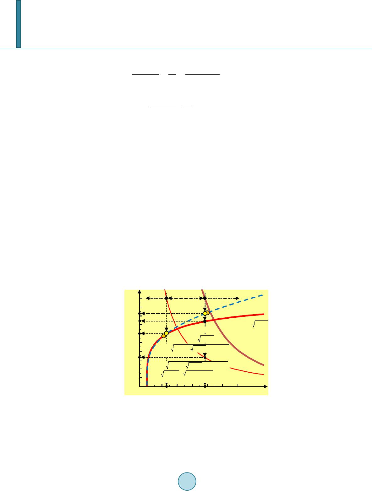 M. Perkovac ∂2Hy(z,t)/∂t2 + ω 2Hy(z,t) = 0. After inclusion of the angular frequency ω = 2πν from Equation (56) we obtain: 2 22 yy 22 0 (,) 1 /2(,) 0 1/ H zteV mc eVHzt A teV mc ∂ 2π − += ∂− . (81) If eV/mc2 << 1, then eV”K = W – U, and Equation (81) becomes 22 y2y 22 0 (,) ()(,) 0 H ztW UHzt tA ∂4π +− = ∂ . (82) 5. Calculation of the Structural Constant s0 Only the structural constant s0 of the atom is unknown in previous expressions. This constant can be determined in several ways, e.g., by measuring two quantities, the voltage V and frequency ν and calculating the action con- stant A0 by Duane-Hunt’s law, i.e., using Equations (15) and (19), [17]. However, here we will use a more direct theoretical calculation, with only one empirical item necessary [18]. Namely, the increase of the nuclear charge in the atom increases atomic number Z. In accordance with Equa- tion (49), the value of structural coefficient σ(χ) = s02/Z is assigned to each atom. So, greater atomic number means a lower structural coefficient σ(χ). On the other hand, there is a critical nuclear charge which ensures stability of the atom [9,19]. In other words, reducing σ(χ) grows instability of the atom. In general, the higher atomic number means less stability (i.e., smaller half-life, or t1/2) of the atom, starting from bismuth 83Bi (Z = 83, t1/2 = 6 × 1026 s, [16]) to ununoctium 118Uuo (Z = 118, t1/2 = 5 ms), [exceptions are atoms of technetium (43Tc, Z = 43, t1/2 = 1.3 × 10¹⁴ s) and prome- thium (63Pm, Z = 63, t1/2 = 5.6 × 10⁸ s )]. For the calculation of structural constant s0 it is enough to find only one associated pair of σ(χ) and Z. The curve σ(χ) has no extremes, Figure 5. Thus it is not easy to find a mentioned pair of σ(χ) and Z. In that sense, a better situation is with the phase velocity uem, specifically with the normalized phase velocity uem(ε*μ*)1/2 = F(χ) of electromagnetic wave in the atom, Figure 5, [9]. Neither of these two curves have extremes, but there is a sharp knee on F(χ) which can be used to determine the structural constant s0. Although there is no theory about the connection between the phase velocity of electromagnetic waves in the atom and the stability of the atoms, it is still possible to use this mathematical benefit of sharp knee for those 2 ([ln(/2/4-1)] / (ln+1/4) Fχ=χ+χχ) 00 ×=()=0.825 40283 = 8.277sσχ Ζ 2 ( )[ln( /2/4-1)](ln+1/4)σχ=χ+χχ Figure 5. Structural coefficient of Lecher’s line σ(χ), norma- lized phase velocity of the electromagnetic wave in the atom F(χ) = uem(ε*μ*)1/2, the first derivative of the normalized phase velocity F'(χ), inverted second derivative of the normalized phase velocity F'' (χ), all versus ratio δ/ρ = χ of the transmis- sion Lecher’s line, consisting of a pair of ideal conducting nonmagnetic parallel wires of radius ρ separated by δ, which represents a model of an atom.  M. Perkovac atoms, in which there is the lower phase velocity of electromagnetic waves that exhibit greater instability. Use of this result will be discussed just a little bit later. The nuclear binding energy per nucleon slightly decreases with increasing atomic number (starting from the first radioactive element bismuth, 83Bi, 7.848 MeV, to the ununoctium, 118Uuo, 7.074 MeV, about 0.31% de- crease for each of the 35 atoms in that area [20]). Physically this means that the boundary between stable and unstable areas is not emphasized. Mathematically it allows that between the two areas there exists so-called transition area, Figure 5. This is, at the moment, the most accurate way to determine the boundary between sta- ble atoms and the others. Indeed, the first unstable atom must be located on that border. This is a key fact to de- termine the structural constant s0 of the atom. Before calculating, we observe the first derivative F ‘(χ) of the curves of normalized phase velocity F(χ) of electromagnetic waves in an atom (Figure 5). When this derivative is greater than 1, it means that the phase ve- locity rapidly declines, that is a zone of unstable atoms (2 < χ < 2.1295317). It should be noted that the situation χ ≤ 2 is theoretically impossible because then there is no Lecher’s line. When the second derivative F’’(χ) of the normalized phase velocity F(χ) is greater than 1, it means that the phase velocity starts to rapidly decline (Figure 5), this is a transition zone (2.129 531 7 < χ < 2.382 788). The border crossing from the transition zone to the stable zone (i.e., χ0 = 2.382 788), in accordance with the experiments, [20], is closest to the bismuth atom. Bismuth atom (83Bi) is the first unstable atom, in the entire chain of stable atoms, which ends with lead (82Pb). The corresponding value of the structural coefficient in that place is σ(χ0) = 0.825402, Figure 5. Bismuth is a chemical element with atomic number Z = 83, with half–life more than a billion times the estimated age of the universe. Even though charges in reality take discrete values (e, 2e, 3e, Ze), theoretical value of Z in Equation (49) can be within the range Zth = 83 ± 1/2. Thus, according to Equation (49) we get the structural constant of the atom [0.825402 × (83 ± 1/2)]1/2, i.e., 8.252 < s0 < 8.302, with a mean value 8.277 and with sample standard deviation ±0.035355 or as a percentage s0 = 8.277 ± 0.43%. Com- paring with the fine structure constant we get s0 = 8.277 56, which is consistent with the calculation performed here (the relative difference is less than 0.0068%). 6. System of the Elements After calculating the structural constants s0 the structural coefficient σ of each element can be determined. For this purpose we use Equations (46) and (49), Figure 6, i.e., 2 20 1 ( )ln1ln 24 4 s Z χχ σχ χ =+−+= . (83) It can be seen that there is a maximal atomic number, 137, just as it is defined in Equation (75). Recently dis- covered element (Z = 118) is ununoctium [Joint Institute for Nuclear Research (JINR) by Yuri Oganessian and his group in Dubna, Russia, 2002]. A century well-known behavior of hydrogen atoms describing Equations (70) and (72) if we put n±1 = n+1 (in the case of n±1 = 1 we get Lyman series, in case of n±1 = 2 Balmer series, n±1 = 3 Paschen series, n±1 = 4 Brackett series, n±1 = 5 Pfund series). Interestingly, the same Equations (70) and (72) describe behavior of neutron, hyperon Λ0 and hyperon Ξ0 if we put n±1 = n–1 (i.e., n±1 = 1/125.886339 for neutron n0, n±1 = 1/137.03543 for hyperon Λ0, n±1 = 1/137.03587 for hyperon Ξ0). This is the reason that all three of these particles are in the same place as hydrogen (Figure 6), [21]. To the similar results regarding the elementary particles otherwise on original way came Giuseppe Bellotti, [22,23]. He was also given new periodic classification of the elements on the basis of standing waves in the atom, using wave equation of potentials of the electron and positron, similar to the Equation (77) of electric and magnetic fields in this paper. 7. Conclusions Maxwell’s equations, together with the Lorentz equations, proved to suffice for the construction of a model of the atom. This model is made by analogy with the transmission line (Lecher’s line). Using this model laws 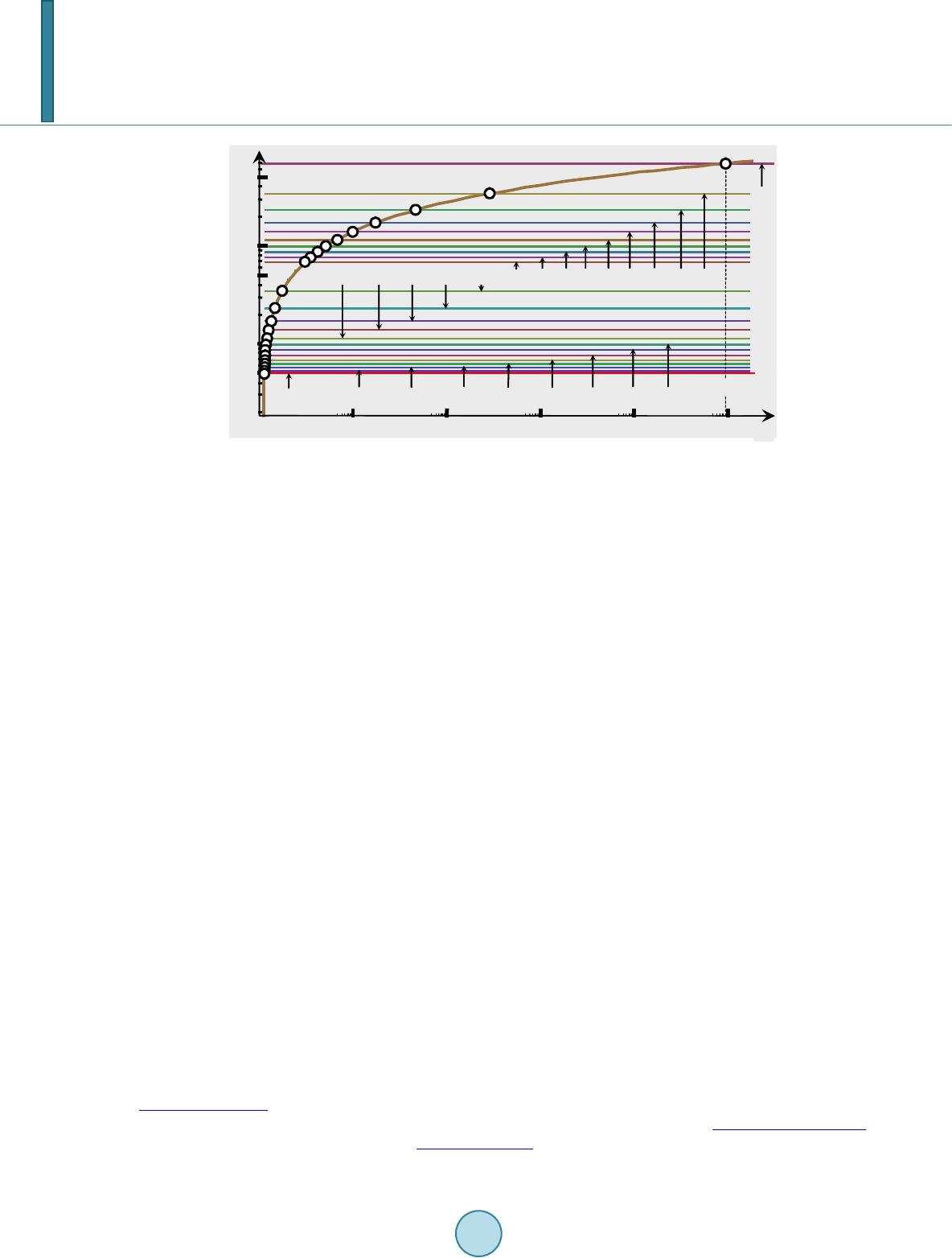 M. Perkovac σ ( 1 H ) = σ ( 5.043 729 881 41×10 29 ) = 68.517 999 540 = s 02 Figure 6. System of the elements, i.e., structural coefficient of Lecher’s line σ vs. parameter χ of Lecher’s line, specifying all known elements, as well as 19 till now undiscovered elements, starting with atomic number 119, up to and including atomic number 137 (log-log scale). Re- cently discovered element, in the second year of two thousand, is ununoctium, Z = 118, Dub- na, Russia (Results from the first 249Cf + 48Ca experiment). Each element has more statio- nary states which are determined with different amount of n±1. So with n±1 = 1 we obtain Ly- man series of radiation of the hydrogen atom, with n±1 = 2 Balmer series, with n±1 = 3 Paschen series, with n±1 = 4 Brackett series, with n±1 = 5 Pfund series. If n±1 = 1/(125.886339) hydro- gen atom takes on the properties of neutron n0, if n±1 = 1/(137.03543) hydrogen atom takes on the properties of hyperon Λ0, and if n±1 = 1/(137.03587) hydrogen atom takes on the proper- ties of hyperon Ξ0. This is why n0, Λ0 and Ξ0 are in the same place where there is hydrogen 1H. A minimal structural coefficient σ min is obtained when the velocity of the electron is equal to the phase velocity of the electromagnetic wave in the atom, i. e., according to Equations (75) and (83) σ min = s02/Zmax = s02/(2s02) = 1/2. The maximal amount of σ arises, according to Equ- ation (83), when the atomic number is the minimal (Z=1), i.e. σ max = s02/Z = s02 = 68.517 999 540. All other elements are within this area. which apply in quantum mechanics are derived, and are performed and Schrödinger’s equation, with the clear meaning of the wave function. The wave function represents the electric or magnetic field strength of the elec- tromagnetic wave in the atom. Using the synchronization of two phenomena within the atom, the electromagnetic wave and the circular mo- tion of electrons, stationary states of atoms are derived. It has been shown that two directions relative to the base state (n = 1) are possible. One is shift of the electron out of the center to the outside (n±1 = n+1; n = 1,2,3…), and the other is a shift in direction to the center of the atom (n±1 = n–1; n = 1,2,3…). The first is a classic, well-known for a hundred years. The latter is a novelty, and it makes possible the formation of neutrons and hyperons using protons and electrons, as is the case by hydrogen. Structural constant of the atoms was determined with the aid of Maxwell’s and Lorentz’s equations. The amount of structural constant 8.27756 is determined by the rapid decline of the phase velocity of the electro- magnetic wave in the atom. It happens to the bismuth atom. Finally, it was found that the atomic number cannot exceed 137, meaning that it is still theoretically possible to detect another 19 so far undiscovered elements. Acknowledgements Wolfram Research, Inc. Mathematica software is used by courtesy of Systemcom, Ltd., Zagreb, Croatia, www.systemcom.hr. The author thanks Ms. Erica Vesic for editing this article in English, Mr. Damir Vuk and Mr. Branko Balon for the useful discussions, Prvomajska TZR, Ltd., Zagreb, Croatia, www.prvomajsk a -tz r.hr and Drives-Control, Ltd., Zagreb, Croatia, www.drivesc.com, for the financial support.  M. Perkovac References [1] Wheeler, J.A. and Fey nman, R.P. (1945) Interaction with the Absorber as the Mechanism of Radiation. Reviews of Modern Physics, 17, 157-181. http://dx.doi.org/10.1103/RevModPhys.17.157 [2] Wheeler, J.A. and Feynman, R.P. (1949) Classical Electrodynamics in Terms of Direct Interparticle Action. Reviews of Modern Physics, 21, 425-433. [3] Perkovac, M. (2002) Quantization in Classical Electrodynamics. Physics Essays, 15, 41-60. http://dx.doi.org/10.4006/1.3025509 [4] Perkovac, M. (2003) Absorption and Emission of Radiation by an Atomic Oscillator. Physics Essays, 16, 162-173. http://dx.doi.org/10.4006/1.3025572 [5] Frankl, D.R. (1986) Electromagnetic Theory. Prentice-Hall, Inc., Englewood Cliffs, New Jersey. [6] Jackson, J.D. (1999) Classical Electrodynamics. 3rd Edition, John Wiley & Sons Inc., New York. [7] Bosanac, T. (1973) Teoretska elektrotehnika 1. Tehnicka knjiga, Zagreb. [8] Haznadar, Z. and Stih, Z. (1997) Elektromagnetizam. Skolska knjiga, Zagreb. [9] Hänsel, H. and Neumann, W. (1995) Physi k. Spektrum Akademischer Verlag, Heidelberg. [10] Perkovac, M. (2012) Maxwell Equations for Nanotechnology. Proceedings of the 35th International Convention of the IEEE MIPRO, Opatija, 21-25 May 2012, 429-436. http://ieeexplore.ieee.org/xpl/freeabs_all.jsp?arnumber=6240683 [11] Rüdenberg, R. (1923) Elektrische Schaltvorgänge. Verlag von Julius Springer, Berlin. [12] Czichos and Association Hütte (1989) Die Grundlagen der Ingenieurwissenschaften. Springer-Verlag, Berlin. [13] Surutka, J. (1971) Elektromagnetika. Gradjevinska knjiga, Beograd. [14] Perkovac, M. (2013) Model of an Atom by Analogy with the Transmission Line. Journal of Modern Physics, 4, 899- 903. http://dx.doi.org/10.4236/jmp.2013.47121 [15] Giancolli, D.C. (1988) Physics for Scientists and Engineers. Prentice Hall, Englewood Cliffs. [16] Page, L. and Adams, N.I. (1940) Electrodynamics. D. Van Nostrand Company, Inc., New York. [17] Perkovac, M. (2010) Statistical Test of Duane-Hunt’s Law and Its Comparison with an Alternative Law. http://arxiv.org/abs/1010.6083 [18] Perkovac, M. (2014) Determination of the Structural Constant of the Atom. Journal of Applied Mathematics and Phys- ics, 2, 11-21. http://dx.doi.org/10.4236/jamp.2014.23002 [19] Benguria, R.D., Loss, M. and Siedentop, H. (2007) Stability of Atoms and Molecules in an Ultrarelativistic Thomas- Fermi-Weizsäcker Model, 1-11. http://dx.doi.org/10.1063/1. 2832620 [20] http://periodictable.com/Isotopes/001.1/index.html [21] http://www.physics.upenn.edu/~pgl/e27/E27.pdf [22] Bellotti, G. (2012) The Hydrogen Atomic Model Based on the Electromagnetic Standing Waves and the Periodic Clas- sification of the Elements. Applied Physics Research, 4, 141-151. http://dx.doi.org/10.5539/apr.v4n3p141 [23] Bellotti, G. (2012) The Ideas Behind the Electromagnetic Atomic Theory. Advances in Natural Science, 5, 7-11. http://cscanada.net/index.php/ans/article/view/j.ans.1715787020120504.2014/3315
|