 Journal of Power and Energy Engineering, 2014, 2, 594-599 Published Online April 2014 in SciRes. http://www.scirp.org/journal/jpee http://dx.doi.org/10.4236/jpee.2014.24080 How to cite this paper: Xing, P.X., et al. (2014) Potential Calculation on the Oil-Gas Pipeline with Geosynthetic Clay Liners Based on BEM. Journal of Power and Energy Engineering, 2, 594-599. http://dx.doi.org/10.4236/jp ee.2014.24080 Potential Calculation on the Oil-Gas Pipeline with Geosynthetic Clay Liners Based on BEM Pengxiang Xing1, Yu Wang1, Hailiang Lu1, Lei Lan1, Xishan Wen1, Shulin Zhang2 1School of Electrical Engineering, Wuhan University, Wuhan, China 2China Liaohe Petroleum Engineering Co. Ltd., Panjin, China Email: pxxing1990@163.com Received Dec emb er 2013 Abstract Put geosynthetic clay liners around underground oil-gas pipelines can reduce the potential dam- age to environment but it will also affect the distribution of cathodic protection current. Geosyn- thetic clay liners can be regarded as anisotropic soil structure and the potential distribution on the pipeline between two adjacent cathodic protection stations was calculated based on boundary element method (BEM). The calculation results indicate that potential distribution on the pipeline with geosynthetic clay liner is lower than before. A 1500 m built pipeline with geosynthetic clay liners was selected to be calculated and to perform field test, which shows that the calculation re- sults tally well with the field test results and the validity of the arithmetic in this paper was veri- fied. Keywords Oil-Gas Pipeline; Geosynthetic Clay Liner; Cathodic Protection; Boundary Element Method (BE M) 1. Introduction Impressed current cathodic protection is one of the most important measures to prevent corrosion and is widely used in underground oil-gas pipeline anticorrosion [1]-[5]. With the development of oil-gas pipeline co nst ruc- tion in China, it has to go through diverse geographical conditions [6]. Put geosynthetic clay liners around un- derground oil-gas pipelines in environmentally sensitive areas can reduce the potential damage to environment when pipeline leakage occurred [7]-[10]. Figure 1 shows the location of geosynthetic clay liners around the oil- gas pip eline. Geosynthetic clay liners can be regarded as anisotropic soil structure around the pipeline because their resis- tivity are different from the soil. Potential distribution on the pipeline between two adjacent cathodic protection station were calculated based on BEM with and without geosynthetic clay liners. A 1500 m built pipeline with geosynthetic clay liners was selected to model and perform feeder test. Potential variation at the cathodic protec- tion current inject point, 200 meters away from one head of the pipeline, was calculated and measured. The cal- culation results tally well with the test results and the validity of the arithmetic in this paper was verified. 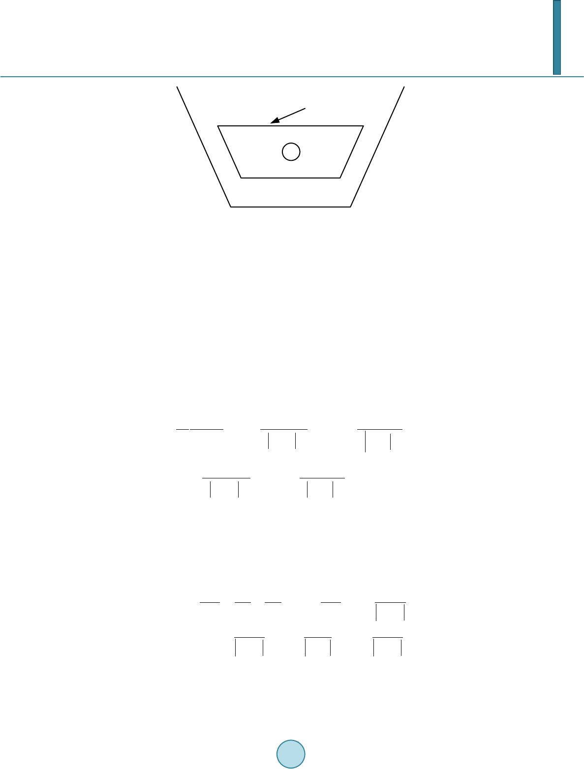 P. X. Xing et al. geosynthetic clay liners pipeline trench Figure 1. Sketch map of geosynthetic clay liners’ construction. 2. Calculation Method of Potential Distribution on the Pipeline First, Geosynthetic clay liners around underground oil-gas pipeline can be model as anisotropic soil structure and the potential anywhere in the soil can be calculated based on BEM. Here’s the basic idea [11]-[16]: Resistivity of geosynthetic clay liners are ρ1 and the soil resistivity is ρ2, Γ is the interface of geosynthetic clay liners and soil, which are marked as Ω1 and Ω2, just as shown in Figure 2. Arithmetic in this paper based on assumptions as follows: (1) Interface Γ is divided into m p arts marked and the surface charge density of every part is , (I = 1, 2,… m), which can be regard as constant if (i = 1, 2,… m) is small enou gh, is the image of . (2) Underground pipeline is divided into r parts marked and the linear charge density of every part is ,their images are . (3) ΔSq is any part on the interface Γ, is unit normal vector and point from Ω1 to Ω2. Surface charge density (q = 1, 2,… m) of any part in the interface Γ is shown as follo ws: 33 11 ' 33 11 ' ˆ ˆ() () 1 2 ˆ ˆ ( )() ll ll ll j jj j mm qq qq ki ql l ll ki SS qq lq nn q qqjq jj jj LL q qj rrn rrn ds ds rr rr rr nrrn dL dL rr rr σσ ηη η πσ σ ξξ = = ≠ = = ′ −⋅ −⋅ −′ =−+ +−′ − ′ − ⋅−⋅ ′ ++ ′ −− ∑∑ ∫∫ ∑∑ ∫∫ (1) where is surface charge density (C/ m2), is linear charge density (C/m), is electrical conductivity (S/m) and E quatio n (1) can be rewrite as follows: 11 0 rm qq jj ll jl AB ξη = = += ∑∑ (2) Potential of arbitrary point on the pipeline (p = 1, 2,… r) is shown as follows: 1/2 2 21 00 1 11 '' 1 ln1 [ 22 4 4 ] ' jp j ll r p pp pj j pL pj jp r mm j ll j ll L SS pj plpl LL dL uaarr dL ds ds r rrrrr ξξ πε πε ξ ηη = ≠ == = = +++ − ′′ + ++ ′ −−− ∑∫ ∑ ∑∑ ∫∫∫ (3) Equation (3) can be rewrite as follows: 11 rm pp jjll p jl C Du ξη = = += ∑∑ (4)  P. X. Xing et al. Figure 2. Sketch map of boundary element method. Rewrite Equations (2) and (4) as matrix form: (5) (6) whe re A, B, C, D are coefficient matrix, U is voltage vector of every section of the pipeline, when the section is small enough its potential can be regard as constant and the potential of section k can be regard as the average potential of the two attached nodes: (7) where V is voltage vector of the pipeline nodes, K is coefficient matrix, if node i connect node j, kij = 0.5, othe r- wis e kij = 0. Replace branch voltage in Equatio n (6) with node voltage in Equatio ns (6) and (7) can be rewrite as follows: (8) Branch current can be divided into two equal parts and allocated to attached nodes, then we can get Equatio n (9). (9) If node j connect branch k, ck,j = 1, other wise ck,j = 0. Equivalent node current dissipate matrix J can be ex- pressed in Eq uation (10). (10) According to electrostatic analogy, electric density on the interface of pipeline and current dissipate can be expressed in Equation (11). (11) Rewrite it as matrix as follows: (12) If the node current vector is F, we can get Equation (13) based on node voltage method in circuit theory. (13) Equation (13) can be rewrite as follows combined Equations (10) and (12). (14)  P. X. Xing et al. Potential and current dissipate of each section of the pipeline can get from the simultaneous solution of Equa- tions (5) (8) and (14). 3. Calculation and Analyse of Pipeline Potential Distribution Model pipeline potential calculation is based on BEM according to part two. The length of the steel underground pipeline is 8500 meters, with a outside diameter 323.9 mm and a thickness 5.6 mm, relative resistance of the pipeline is 10 and the relative permeability is 636; soil resistivity is 593 Ω·m and the resistivity of geosynthetic clay liners is 200 Ω·m with a thickness 5 cm. Cathodic protection current at two ends of the pipeline are 50 mA, 100 mA, 150 mA and 200 mA. The varied potential distribution on the pipeline with and without geosynthetic clay liners are shown in Figure 3, represented by and separately, where l is the length of the pipeline (m), ΔU is the varied potential (V). Calculation results indicate that the varied potential increased with cathodic protection current and the varied potential distribution on the pipeline seems to be inverted U, namely higher in the two ends and lower in the middle, and the voltage variation gradient in the two ends are much bigger than middle parts. Potential distribu- tion on the pipeline with geosynthetic clay liners has overall declined compared to it used to be. The ratio of ΔU and its previous potential is defined as potential decrease percentage and the maximum value 10% occured at the two ends of the pipeline, namely the cathodic protection current inject points. So cathodic protection current should increased properly when geosynthetic clay liners are put around the underground pipeline. 4. Feeder Test and Analyse In order to verify the accuracy of the arithmetic in this paper, field feeder test was performed in China and Myanmar oil-gas pipeline Jinning extension, the test pipeline is 1500 meters long and has been covered with geosynthetic clay liners. Feeder test method [17]-[19] is shown in Figure 4. Temporary anode bed in the field test was made up by 6 angle steels with a length of 1 meter, which are pa- rallel co nne cted with each other, the temporary anode bed was 100 meters away in vertical distance from the test pipeline. Anode of the DC power was linked to the temporary anode bed and the cathode of the DC power was linked to the pipeline by a test pile 200 meters away from one head of the pipeline. Spontaneous potential of the 01000 2000 3000 4000 5000 6000 7000 8000 -0.05 -0.045 -0.04 -0.035 -0.03 -0.025 -0.02 -0.015 -0.01 -0.005 0 △U/V l/m 010002000 30004000 5000 6000 70008000 -0.1 -0.09 -0.08 -0.07 -0.06 -0.05 -0.04 -0.03 -0.02 -0.01 0 l/m △ U/V (a) (b) 010002000 30004000 5000 600070008000 -0.16 -0.14 -0.12 -0.1 -0.08 -0.06 -0.04 -0.02 0 △ U/V l/m 01000 2000 3000 4000 5000 6000 7000 8000 -0.2 -0.18 -0.16 -0.14 -0.12 -0.1 -0.08 -0.06 -0.04 -0.02 0 △ U/V l/m (c) (d) Figure 3. Potential distribution on the pipeline with different cathodic protection current.  P. X. Xing et al. 1—underground pipeline; 2—geosynthetic clay liners 3—connected cable; 4—temporary anode 5—copper sulfate reference electrode Figure 4. Sketch map of pipeline feeder test. pipeline was −1 V and the pipeline potential became −1.2 V when adjust cathodic protection current to 120 mA, potential variation ΔU = −0.2 V. Based on the arithmetic in this paper, the calculation result of cathodic protec- tion current is 113 mA when potential variation ΔU at the current inject point is −0.2 V, relative error is 5.83%, which indicate that the calculation result agree well with the test result. 5. Conclusion Potential distribution on the pipeline with geosynthetic clay liners was calculated based on BEM in this paper and it indicated that the pipeline potential get a slight decline when geosynthetic clay liners were put around the pipeline. Both the maximum potential variation and the maximum potential decrease percentage were occurred at the cathodic protection current inject point. Validity of the arithmetic in this paper to calculate potential dis- tribution on the pipeline with geosynthetic clay liners was verified by the comparison with field test. References [1] Bake men, W.V., Siwenke , W. and Pulizi, W. (20 05 ) Cathodic Protection Manual. Translated by Hu, S.X. and Wang, X.N. Chemical Industry Press, Beijing. [2] (2000) National Petroleum and Chemical Industry. People ’s Republic of China Oil and Gas Industry Standards SY/T0036-2000: Standard for the Impressed Current Cathodic Protection of Und er-Ground Steel Pipeline. Petroleum Industry Press, Beijing. [3] Hu, S.X . (2004) Present Situation and Forecast about Pipeline Cathodic Protection. Corrosion and Protection, 25, 93-101. [4] Li n , X.Y., Wu, M., Cheng, H. L. , Long, S.H. and Wang, P. (2011) Corrosion Mechanism of Buried Oil Pipelines and Protection. Contemporary Chemical Industry, 40, 53-59. [5] Nian , D.H. (2012) Application Analysis about Cathodic Protetion Technology at Present. Corrosion and Protection, 15, 68-70. [6] Li , Z.L. , Cui, G., Shang, X.B. and Liu , Y. (20 13 ) Defining Cathodic Protection Potential Distribution of Long Distance Pipeline with Numerical Simulation. Corrosion and Protection, 34, 468-470. [7] Wan g, Z. (2002) Application Research of Abroad Geosynthetic Materials. Modern Knowledge Press, Hong Kong. [8] Han , J.Y. and Shen , D.X. (20 03) Development and Application of Geosynthetic in Engineering. China Building Mate- rials Industry Press, Beijing. [9] Li , Z.B. (2007) Geotextiles Bentonite Clay Seepage Control Effectiveness Research and Related Mechanism Analyses. Ph.D. Thesis, Tongji University, Shanghai. [10] Roberto, Galiasso and Tailleu (2007) Effect of Recycling the Unconverted Residue on a Hydrocracking Catalyst Oper- ating in an Ebullated Bed Reactor. Fuel Processing Technology, 88, 779-785 . [11] Zhang, Y.Z., Wang, Y.M. and Liu , L.L. (2011 ) Numerical Simulation Technology in the Application of Long-Distance Pipeline Cathodic Protection. Corrosion and Protection, 32, 969-971. [12] Chen , S.Y., Wu, X.C. and Jiang, G.Y. (2008) Numerical Calculation Method on Current and Potential of Impressed Current Cathodic Protection System for Pipeline. Journal of Petrochemical Universities, 21, 75-78. [13] Zhang, F., Chen, H.Y. and Li, G. D. (2011) Numerical Simulation Applied in the Pipeline and Station. Oil and Gas Storage and Transmission, 30 , 208 -212.  P. X. Xing et al. [14] Zhang, Z. and Wen, X.S. (2010) Boundary Element Analysis on Grounding Systems in Soil with Arbitrary Massive Text u r e. Power System Technology, 34, 1 70-17 4. [15] Gu o , W., Li, X.P., Wen, X.S., Xin g, P.X ., Jiang, Z.P. , Wang, Y., et al. (2013) Research on Applying Boundary Ele- ment Method to Grounding Grid in Soil with Massive Texture. Power System Technology, 37, 1414-1419. [16] P eng, Y.L. and Wang, J.Q. (1995) Application of BEM in Foundation Earth Field. High Voltage Engineering, 21 , 79-82. [17] Kong, F.R. (2004 ) Requirement and Construction of the Auxiliary Anode in Cathodic Protection of Oil Pipeline. Cor- rosion and Protection, 25, 161-163. [18] Liu , S.F. (2013 ) Pipeline’s Cathodic Protection Testing. Total Corrosion Control, 27, 31-34. [19] You, S.Y., Zhao, Y.F., Ma, B. and Ding, Z.N. (2011) Error Analysis and Countermeasure about Cathodic Protection Potential. Corrosion and Protection, 32, 969-971 .
|