Paper Menu >>
Journal Menu >>
 Applied Mathematics, 2011, 2, 444-451 doi:10.4236/am.2011.24056 Published Online April 2011 (http://www.SciRP.org/journal/am) Copyright © 2011 SciRes. AM Moments of Discounted Dividend Payments in the Sparre Andersen Model with a Constant Dividend Barrier* Jiyang Tan1, Lin Xiao2, Shaoyue Liu1, Xiangqun Yang2 1Department of Stat i st i c s, Xiangtan University, Xiangtan, China 2Department of Mat hem at ic s, Hunan Normal Un iversity, Changsha, China E-mail: tanjiyang15@163.com Received December 23, 2010; revised February 14, 2011; accepted February 26, 2011 Abstract We consider the Sparre Andersen risk process in the presence of a constant dividend barrier, and propose a new expected discounted penalty function which is different from that of Gerber and Shiu. We find that ite- ration mothed can be used to compute the values of expected discounted dividends until ruin and the new penalty function. Applying the new function and the recursion method proposed in Section 5, we obtain the arbitrary moments of discounted dividend payments until ruin. Keywords: Sparre Andersen Model, Expected Discounted Penalty Function, Constant Dividend Barrier, Recursion, Iteration 1. Introduction The dividend problem in risk theory was brought out initially by De Finetti [1] and has been studied exten- sively in many literatures by now. Much of the literature on dividend theory is concentrated on the classical risk model, in which claims occur as a Poisson process. For the classical risk model with a barrier strategy, Lin et al. [2] studied the Gerber-Shiu discounted penalty function at ruin; Dickson and Waters [3] studied arbitrary mo- ments of the discounted sum of dividend payments until ruin; Gerber et al. [4] recently developed methods for estimating the optimal dividend barrier. The surplus process is not necessarily a compound Poisson process. Andersen [5] lets claims occur accord- ing to a more general renewal process. Since then, Sparre Andersen risk model was studied extensively. For some recent contributions to Sparre Andersen risk models with a dividend barrier, see [6-8]. It is worth mentioning that Albrecher et al. [8] studied a class of Sparre Andersen risk models with generalized Erlang(n) waiting times in the presence of a constant dividend barrier b, and gained some results on the distribution of dividend payments until ruin. It is natural to ask for developing some me- thods to get the distribution or moments of discounted dividend payments in an arbitrary Sparre Andersen mo- del. In this paper, we consider the Sparre Andersen model with arbitrary distributed waiting times in the presence of a constant dividend barrier b. The analysis is focused on the evaluation of the new expected discounted penalty function defined in Section 2, which will permit us to obtain arbitrary moments of discounted dividend pay- ments by applying the proposed recursion method. 2. The Model Consider the Sparre Andersen risk model, which is given by 1 N i t i Utu ctStu ctX (2.1) where 0u is the initial surplus, c is a constant pre- mium rate, St is the aggregate claim up to time t, N(t) is the number of claims occurring in (0,t], and i X is the ith claim. Let 12 ,,MM denote the inter-claim times, and assume that 1 . n nk k LM We assume that ,1 n Xn and ,1 n Mn are in- dependent sequences of i.i.d. non-negative random va- riables. ,1 n Xn have a common distribution *Supported by the Natural Sciences Foundation of China (grant No. 10871064), and by Scientific Research Funds of Hunan Provincial Education Department (08C883), and Hunan Provincial Science and Technology Department (2009FJ3141).  J. Y. TAN ET AL. Copyright © 2011 SciRes. AM 445 1 Pr F xXx with (0) 0F, and ,1 n Mn have a common distribution 1 () PrGxM x with (0) 0G. Assume 1 EM . The risk process (2.1) is now modified by introducing a constant dividend barrier b 0b, i.e. whenever the surplus process reaches the level b, the premium income is paid out as dividends to shareholders and the modified surplus process remains at level b until the occurrence of the next claim. Let b Ut denote the modified sur- plus process, and the random variable D (u,b) denote the sum of the discounted dividend payments until ruin (with force of interest 00 ). In the sequel we will be inter- ested in the kth moment of the sum of discounted divi- dend payments ,| 0,1,2,. kk b WuEDubUu k Let 1 bb WuWu, which is the expectation. We will always assume that 0ub. Let the time of ruin for this modified surplus process () b Ut be inf0:0 otherwise bb TTut Ut Obviously, T must be some i L. Define the stochastic time by () inf:,1. bii uLULbi For 0,x let v(x) be a non-negative measurable function. For 00 we define a new expected dis- counted penalty function by 0,0 buEevUI TUuub (2.2) where I is the indicator function. The function bu is similar to (but different from) Gerber-Shiu expected discounted penalty function. Let S denote the space of real-valued measurable func- tions on [0,b]. Choosing the metric defined by 0, d,sup, ,, ub x yxuyuxyS ,SSdis complete metric space. Obviously, b Wu and bu are contained within S because of the mea- surable property of vx and the monotone property of b Wu . 3. The Expectation of Discounted Dividends Until Ruin Define an operator :TS S by 0 0 00 1 0 dd dd, bu cuctt bt buc Tffuctx eFxGt f bxeFxGt D (3.1) where f = f(u) is an arbitrary function in S, and 1 D 0 0 0 00 0 1d, 0 1d, 0 ub t c bu c bu c cbuc eG eGt c bu ub GctGt c (3.2) Theorem 1. Under the assumption that 1Fb or 00 , the function b Wu is equal to lim, 0. n bn WuTfub (3.3) As an approximation of , b Wu n Tf u satisfies 0, 0, supsup , 1 n n b ub ub Tf uWufuTf u (3.4) where 0 0d. t F beGt Proof. Ruin can not occur in (0, 1 L) and the expecta- tion of the discounted dividends paid out in this period is 1 D. By the renewal argument we have 01 111 , L bb WuEeW ucLbXD namely, 0 0 () 00 1 ()/0 ()d d d, bu cuctt bb bt b buc WuWu ctxeFxGt Wbxe dFxGtD (3.5) which is an integral equation for . b Wu Since , b WuS the Equation (3.5) can be rewritten as . bb WuTW u (3.6) For arbitrary ,,fg S we have 0, d, sup ub Tf Tg 0 00 d()d bu cuctt f uctx guctxeFxGt 0 ()/0 |( )()|d()d() bt buc f bx gbxeFxGt 0 () 00 0, 0, supsupd()d() bu cuctt ub ub f ugue FxGt 0 ()/0 d()d() bt bu ceFxGt 0 00 d,d d bt f geFxGt which leads to 0 0 (,) (,)()d(). t dTfTgd f gFbeGt (3.7)  J. Y. TAN ET AL. Copyright © 2011 SciRes. AM 446 Thus, T is a contraction on S if F(b) < 1 or 00 (see [9]). (3.3) and (3.4) follow. Note that when b = 0 we have, for 00 , 0 00 0 01 d, t c WeGt (3.8) and for 00 , 01 0.WcEM Theorem 1 gives an iteration procedure by which we can obtain approximations to b Wu and error bounds. In order to gain more information about the sum of dis- counted dividend payments until ruin, we discuss the new expected discounted penalty function in Section 4. 4. Expected Discounted Penalty Function Define an integral operator as follows: 00 / dd d,. bu cuctt t bu c Tffuctx eFxG t evuctGtf S (4.1) Theorem 2. The penalty function bu is the solu- tion of the integral equation . bb uTu (4.2) And under the assumption that F(b) < 1 or G(b/c) < 1 or 0, the penalty function bu is the unique solution and equal to lim , n bn uTfu (4.3) where f is an arbitrary real-valued measurable function. Proof. The discrete time process ,0,1, bn UL n has stationary and independent increments. By the re- newal argument, we have the integral Equation (4.2). The uniqueness and the result (4.3) are due to the fact that T is a contraction under the conditions F (b) < 1 or G (b/c) < 1 or 0. In fact, for arbitrary real-valued measurable functions y(u) and z(u) on [0,b], we have 0, 0, sup sup ub ub Ty Tz 00 dd bu cuctt yu ctxzu ctxeFxGt 0 [0,][0, ] sup supd bu ct ub ub yuzueFu ctGt 0 0, supd , bc t ub yuzu FbeGt where 0d1. bc t Fbe Gt The results are proven. Remark. 1) Obviously, when u = b we can obtain the explicit expression 0 ()d . t bbevbctGt (4.4) 2) According to Theorem 2, we can obtain the ap- proximation of bu by the iteration method. As an approximation of , bu n Tf satisfy 0, 0, supsup , 1 n n b ub ub Tf uufuTfu (4.5) where 0 0, sup d bu ct ub eFuctGt .The error bound (4.5) can be used for estimating the number of steps necessary to reach a given accuracy. Now, we give some examples of dividend-related quantities (such as the probability of the event bb uTu , the kth moment of the discounted divi- dends paid out in time period 0, , and the distribution function of the sum of the dividends paid out in time pe- riod 0, , etc.) to illustrate applications of Theorem 2. Example 4.1. Letting v(x) = 1 and 0, we have Pr . bbb uuTu The contraction T is defined by 00 dd 1, . bu cuct TfufuctxFxGt bu GfS c (4.6) For any real-valued measurable function f on [0,b], we have Prlim . n bbn uTuTf (4.7) From (4.4), it is easily seen that Pr 1 bb bTb . (4.8) Example 4.2. Letting v(x) = 1 and 0, we have . bbb uEeI uTu Let Ru denote this function. Note that 0Pr . bb Ruu Tu Here, the contraction T is defined by 00 dd d. bu cuctt t buc Tfu efuctxFxGt eGt (4.9) Choosing f = 0, we have limd . nt buc n RuTeGt (4.10) The error estimate is  J. Y. TAN ET AL. Copyright © 2011 SciRes. AM 447 0 0, supd . 1 n nt ub Tf uRueGt (4.11) By (4.4), we have 0 ()d (). t RbeGt (4.12) Example 4.3. The insurer will continuously pay divi- dends in time period ,Ubc at rate c when T . Set 0 0 1. xb c c wx e Then, the present value of these dividends is 0.ewU For arbitrary 0,1,i, letting i vxw xand 0, yields , i bbb uEewUIuTu which we denote by ,. i A u The contraction T is defined by 00 dd d. bu cuctt ti bu c Tfu efuctxFxGt ewuctGt (4.13) Choosing 0fu, we have ,limd . nti ibuc n A uT ewuctGt (4.14) The error estimate is 0 , 0, 0 0 sup 1d . 1 n i ub in i t t i Tf uAu cee Gt (4.15) Note that if 0 i , then 0 ,,iii A uAu is the ith moment of the discounted dividends paid out in the period 0, ; if 0,i i.e. 0,vxw x then ,0 . A uRu In addition, it should be pointed out that ,0d. ti i A bewuctGt (4.16) Example 4.4. Letting 0, and vxIx bz for arbitrary 0z, we have Pr, , buU bzT which is the distribution function of the cumulative divi- dends in time period /, .Ubc We de- note this distribution function by ,.uz The contrac- tion T is defined by 00 dd . bu cuct TfufuctxFxGt buz bu GG cc (4.17) Choosing 0fu , we have ,lim. n n buz bu uzT GG cc (4.18) The error estimate is 0, sup ,, 1 n n ub bz Tf uuzGc (4.19) where / 0 0, supd . bu c ub F uctGt 5. The kth Moment of Discounted Dividend Payments Until Ruin In this section, we use 1u (or 1 ) instead of bu and use 1 Tu (or 1 T) instead of . b Tu If ruin doesn’t occur at time 1u and 12b Uu (2 0ub ), we view the process as “starting again” with “initial surplus” 2 u, and similarly to the definitions of b Tu and bu , define the stochastic times 222 TTu and 222 u respectively for the new pro cess 2b Uu. If ruin doesn’t occur at 2 either, similarly we define 333 TTu and 333 u . Ap- plying repeatedly the idea of “starting again”, we can define two sequences of mutually independent random variables ,1 i Ti and ,1 ii . Suppose that the claim amount at i is 1i X. Then, ii ubX (2i). Further, suppose that 01 111 ,eI T 0,2. i iii i IXb eITi Then, i (2i) are i.i.d. random variables and inde- pendent of 1 . According to Example 2 in Section 4, we have 0 1 kk ERu and 0 0 222 0 d. kk b k EEIXbRbX RbxFx (5.1) We denote 2 k E by k R. Assume that 01 1111 ,ewUI T 0,2, i iiii i IXb ewUITi which is the “present value” of the dividends paid in time period 0, i in the (i − 1)th “starting again” process. Obviously, i 2i are i.i.d. random variables and random vectors 11 , , 22 , , are mutually in- dependent. According to Example 3 in Section 4, we have 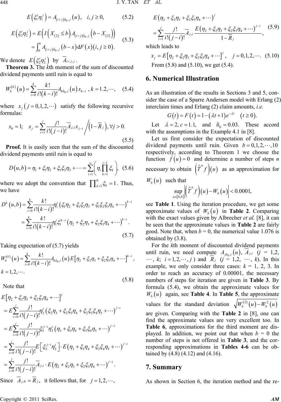 J. Y. TAN ET AL. Copyright © 2011 SciRes. AM 448 0 11 ,,,0, ij ij j EAuij (5.2) 0 0 22 2,2 , 0 d,0. ij ij j b ij j EEIXbAbX AbxFxij (5.3) We denote 22 ij E by ,ijj A. Theorem 3. The kth moment of the sum of discounted dividend payments until ruin is equal to 0, 0 !,1.2,, !! k k bkiki i k WuA uxk iki (5.4) where 0,1, 2, j xj satisfy the following recursive formulas: , 0 1 ! 1;1, 0. !! j ji j jji i j xxAx Rj iji (5.5) Proof. It is easily seen that the sum of the discounted dividend payments until ruin is equal to 1 112 123 11 ,, i ik ik Dub (5.6) where we adopt the convention that 0 11 k k . Thus, we have 1 121231234 0 112 23 234 0 ! ,!! ! . !! kki ki i kki iki i k Dub iki k iki (5.7) Taking expectation of (5.7) yields 0,223234 0 !, !! 1, 2,. kki k bki i k WuA uE iki k (5.8) Note that 223234 j E 2 232342345 0 ! !! j j i i i j Eiji 223 34345 0 ! !! j j i jii i j Eiji 223 34 345 0 ! !! j j i jii i jEE iji ,223234 0 !. !! j j i ji i jAE iji Since ,0 , j j A R it follows that, for 1,2,,j 223234 223234 , 1 !, !! 1 j j i j ji j i E E jA iji R (5.9) which leads to 223234 ,0,1,2,. j j xE j (5.10) From (5.8) and (5.10), we get (5.4). 6. Numerical Illustration As an illustration of the results in Sections 3 and 5, con- sider the case of a Sparre Andersen model with Erlang (2) interclaim times and Erlang (2) claim amounts, i.e. 11 0. t Gt Fttet Let 2, 1.1,c and 00.03. These accord with the assumptions in the Example 4.1 in [8]. Let us first consider the expectation of discounted dividend payments until ruin. Given 0,1, 2,,10b respectively, according to Theorem 1 we choose the function 0fu and determine a number of steps n necessary to obtain n Tf u as an approximation for b Wu such that 0, sup 0.0001, n b ub Tf uWu see Table 1. Using the iteration procedure, we get some approximate values of b Wu in Table 2. Comparing with the exact values given by Albrecher et al. [8], it can be seen that the approximate values in Table 2 are fairly good. Note that, when b = 0, the numerical value 1.076 is obtained by (3.8). For the kth moment of discounted dividend payments until ruin, we need compute 0,, ji A u , j i A (j = 1,2, , k; 1, 2,,ij ) and j R (j = 1,2, , k). In this example, we only consider three cases: k = 1, 2, 3. In order to reach an accuracy of 0.00001, the necessary numbers of steps for iteration are given in Table 3. By formula (5.4), we obtain the approximate values for b Wu again, see Table 4. In Table 5, the approximate values for the standard deviation 22 bb WuWu are given. Comparing with the Table 2 in [8], one can find the approximate values are very excellent too. In Table 6, approximations for the third moment are dis- played. In addition, we point out that when b = 0 the number of steps is not offered in Table 3, and the cor- responding approximations in Tables 4-6 can be ob- tained by (4.8) (4.12) and (4.16). 7. Summary As shown in Section 6, the iteration method and the re- 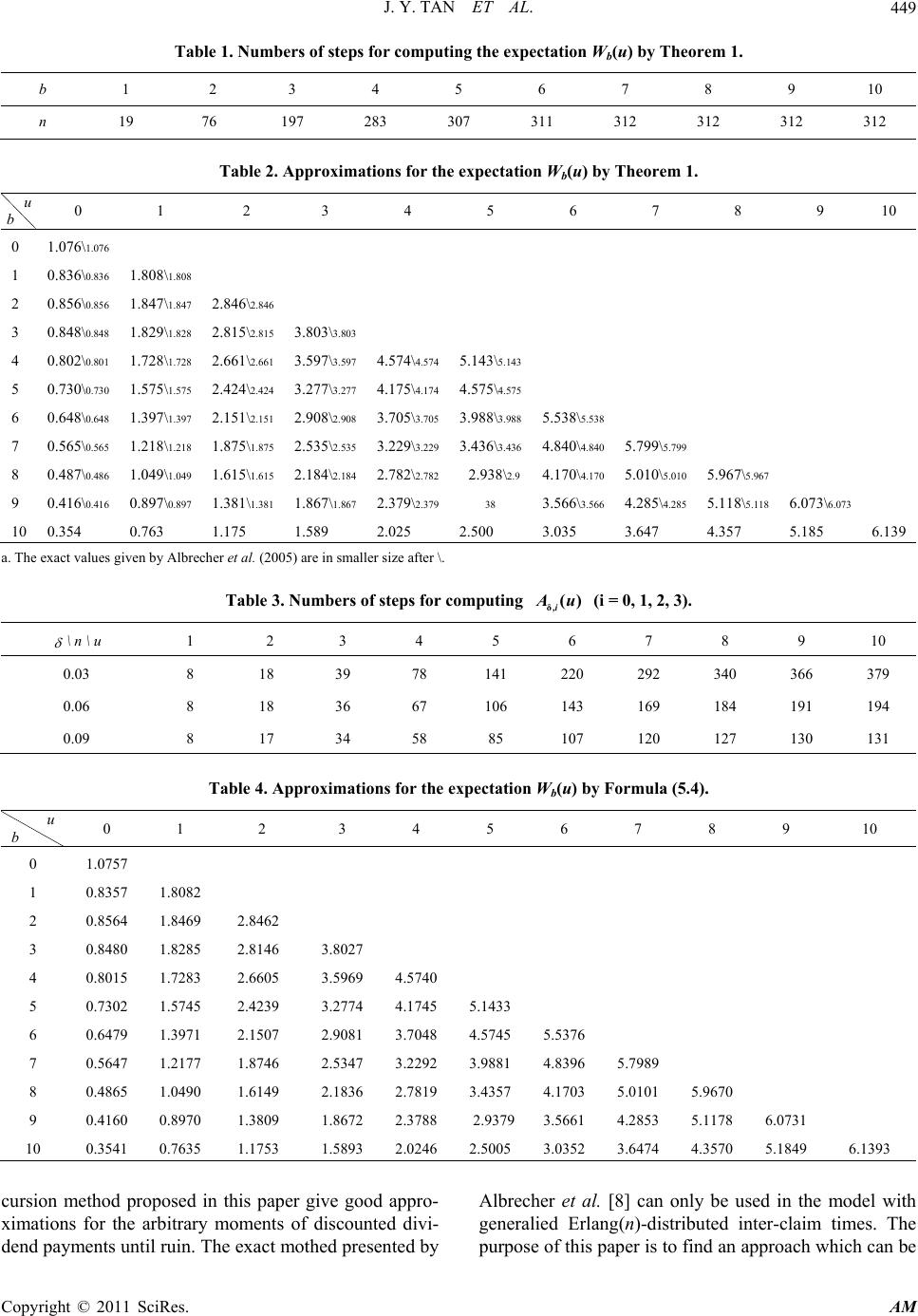 J. Y. TAN ET AL. Copyright © 2011 SciRes. AM 449 Table 1. Numbers of steps for computing the expectation Wb(u) by Theorem 1. b 1 2 3 4 5 6 7 8 9 10 n 19 76 197 283 307 311 312 312 312 312 Table 2. Approximations for the expectation Wb(u) by Theorem 1. u b 0 1 2 3 4 5 6 7 8 9 10 0 1 2 3 4 5 6 7 8 9 10 1.076\1.076 0.836\0.836 0.856\0.856 0.848\0.848 0.802\0.801 0.730\0.730 0.648\0.648 0.565\0.565 0.487\0.486 0.416\0.416 0.354 1.808\1.808 1.847\1.847 1.829\1.828 1.728\1.728 1.575\1.575 1.397\1.397 1.218\1.218 1.049\1.049 0.897\0.897 0.763 2.846\2.846 2.815\2.815 2.661\2.661 2.424\2.424 2.151\2.151 1.875\1.875 1.615\1.615 1.381\1.381 1.175 3.803\3.803 3.597\3.597 3.277\3.277 2.908\2.908 2.535\2.535 2.184\2.184 1.867\1.867 1.589 4.574\4.574 4.175\4.174 3.705\3.705 3.229\3.229 2.782\2.782 2.379\2.379 2.025 5.143\5.143 4.575\4.575 3.988\3.988 3.436\3.436 2.938\2.9 38 2.500 5.538\5.538 4.840\4.840 4.170\4.170 3.566\3.566 3.035 5.799\5.799 5.010\5.010 4.285\4.285 3.647 5.967\5.967 5.118\5.118 4.357 6.073\6.073 5.185 6.139 a. The exact values given by Albrecher et al. (2005) are in smaller size after \. Table 3. Numbers of steps for computing δ() ,i Au (i = 0, 1, 2, 3). \ n \ u 1 2 3 4 5 6 7 8 9 10 0.03 8 18 39 78 141 220 292 340 366 379 0.06 8 18 36 67 106 143 169 184 191 194 0.09 8 17 34 58 85 107 120 127 130 131 Table 4. Approximations for the expectation Wb(u) by Formula (5.4). u b 0 1 2 3 4 5 6 7 8 9 10 0 1 2 3 4 5 6 7 8 9 10 1.0757 0.8357 0.8564 0.8480 0.8015 0.7302 0.6479 0.5647 0.4865 0.4160 0.3541 1.8082 1.8469 1.8285 1.7283 1.5745 1.3971 1.2177 1.0490 0.8970 0.7635 2.8462 2.8146 2.6605 2.4239 2.1507 1.8746 1.6149 1.3809 1.1753 3.8027 3.5969 3.2774 2.9081 2.5347 2.1836 1.8672 1.5893 4.5740 4.1745 3.7048 3.2292 2.7819 2.3788 2.0246 5.1433 4.5745 3.9881 3.4357 2.9379 2.5005 5.5376 4.8396 4.1703 3.5661 3.0352 5.7989 5.0101 4.2853 3.6474 5.9670 5.1178 4.3570 6.0731 5.1849 6.1393 cursion method proposed in this paper give good appro- ximations for the arbitrary moments of discounted divi- dend payments until ruin. The exact mothed presented by Albrecher et al. [8] can only be used in the model with generalied Erlang(n)-distributed inter-claim times. The purpose of this paper is to find an approach which can be 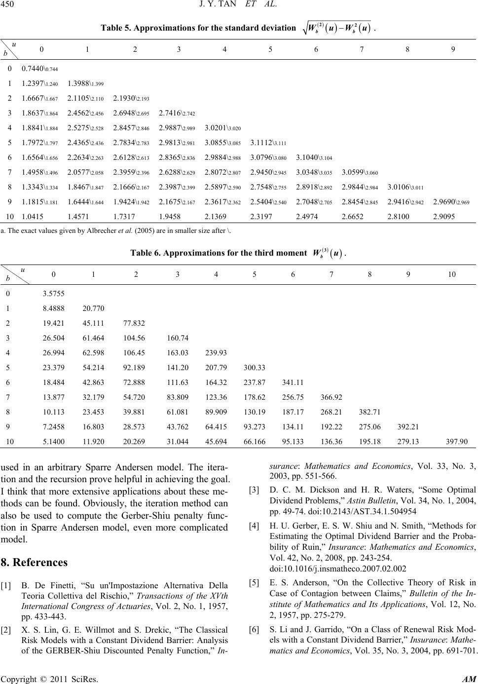 J. Y. TAN ET AL. Copyright © 2011 SciRes. AM 450 Table 5. Approximations for the standard deviation 22 bb WuWu. u b 0 1 2 3 4 5 6 7 8 9 0 1 2 3 4 5 6 7 8 9 10 0.7440\0.744 1.2397\1.240 1.6667\1.667 1.8637\1.864 1.8841\1.884 1.7972\1.797 1.6564\1.656 1.4958\1.496 1.3343\1.334 1.1815\1.181 1.0415 1.3988\1.399 2.1105\2.110 2.4562\2.456 2.5275\2.528 2.4365\2.436 2.2634\2.263 2.0577\2.058 1.8467\1.847 1.6444\1.644 1.4571 2.1930\2.193 2.6948\2.695 2.8457\2.846 2.7834\2.783 2.6128\2.613 2.3959\2.396 2.1666\2.167 1.9424\1.942 1.7317 2.7416\2.742 2.9887\2.989 2.9813\2.981 2.8365\2.836 2.6288\2.629 2.3987\2.399 2.1675\2.167 1.9458 3.0201\3.020 3.0855\3.085 2.9884\2.988 2.8072\2.807 2.5897\2.590 2.3617\2.362 2.1369 3.1112\3.111 3.0796\3.080 2.9450\2.945 2.7548\2.755 2.5404\2.540 2.3197 3.1040\3.104 3.0348\3.035 2.8918\2.892 2.7048\2.705 2.4974 3.0599\3.060 2.9844\2.984 2.8454\2.845 2.6652 3.0106\3.011 2.9416\2.942 2.8100 2.9690\2.969 2.9095 a. The exact values given by Albrecher et al. (2005) are in smaller size after \. Table 6. Approximations for the third moment 3 b Wu. u b 0 1 2 3 4 5 6 7 8 9 10 0 1 2 3 4 5 6 7 8 9 10 3.5755 8.4888 19.421 26.504 26.994 23.379 18.484 13.877 10.113 7.2458 5.1400 20.770 45.111 61.464 62.598 54.214 42.863 32.179 23.453 16.803 11.920 77.832 104.56 106.45 92.189 72.888 54.720 39.881 28.573 20.269 160.74 163.03 141.20 111.63 83.809 61.081 43.762 31.044 239.93 207.79 164.32 123.36 89.909 64.415 45.694 300.33 237.87 178.62 130.19 93.273 66.166 341.11 256.75 187.17 134.11 95.133 366.92 268.21 192.22 136.36 382.71 275.06 195.18 392.21 279.13 397.90 used in an arbitrary Sparre Andersen model. The itera- tion and the recursion prove helpful in achieving the goal. I think that more extensive applications about these me- thods can be found. Obviously, the iteration method can also be used to compute the Gerber-Shiu penalty func- tion in Sparre Andersen model, even more complicated model. 8. References [1] B. De Finetti, “Su un'Impostazione Alternativa Della Teoria Collettiva del Rischio,” Transactions of the XVth International Congress of Actuaries, Vol. 2, No. 1, 1957, pp. 433-443. [2] X. S. Lin, G. E. Willmot and S. Drekic, “The Classical Risk Models with a Constant Dividend Barrier: Analysis of the GERBER-Shiu Discounted Penalty Function,” In- surance: Mathematics and Economics, Vol. 33, No. 3, 2003, pp. 551-566. [3] D. C. M. Dickson and H. R. Waters, “Some Optimal Dividend Problems,” Astin Bulletin, Vol. 34, No. 1, 2004, pp. 49-74. doi:10.2143/AST.34.1.504954 [4] H. U. Gerber, E. S. W. Shiu and N. Smith, “Methods for Estimating the Optimal Dividend Barrier and the Proba- bility of Ruin,” Insurance: Mathematics and Economics, Vol. 42, No. 2, 2008, pp. 243-254. doi:10.1016/j.insmatheco.2007.02.002 [5] E. S. Anderson, “On the Collective Theory of Risk in Case of Contagion between Claims,” Bulletin of the In- stitute of Mathematics and Its Applications, Vol. 12, No. 2, 1957, pp. 275-279. [6] S. Li and J. Garrido, “On a Class of Renewal Risk Mod- els with a Constant Dividend Barrier,” Insurance: Mathe- matics and Economics, Vol. 35, No. 3, 2004, pp. 691-701.  J. Y. TAN ET AL. Copyright © 2011 SciRes. AM 451 doi:10.1016/j.insmatheco.2004.08.004 [7] M. M. Claramunt, M. Marmol and R. Lacayo, “On the Probability of Reaching a Barrier in an Erlang(2) Risk Process,” Working Paper No. 24, Universitat Autonoma de Barcelona, Cerdanyola del Vallès, 2004. [8] H. Albrecher, M. Mercgravee Claramunt and M. Marmol, “On the Distribution of Dividend Payments in a Sparre Andersen Model with Generalized Erlang(n) Interclaim Times,” Insurance: Mathematics and Economics, Vol. 37, No. 2, 2005, pp.324-334. doi:10.1016/j.insmatheco.2005.05.004 [9] Erwin Kreyszig, “Introductory Functional Analysis with Applications,” John Wiley & Sons, Hoboken, 1978, pp. 299-302. |