 Journal of Geoscience and Environment Protection, 2014, 2, 134-142 Published Online April 2014 in SciRes. http://www.scirp.org/journal/gep http://dx.doi.org/10.4236/gep.2014.22019 How to cite this paper: Mudragaddam, M. et al. (2014). Prediction of CO2 and H2S Emissions from Wastewater Wet Wells. Journal of Geoscience and Environment Protection, 2, 134-142. http://dx.doi.org/10.4236/gep.2014.22019 Prediction of CO2 and H2S Emissions from Wastewater Wet Wells Madhuri Mudragaddam, Bhaskar Kura, Amrita Iyer, Elena Ajdari Civil & Environmental Engineering, University of New Orleans, Louisiana, USA Email: bkura@uno.edu Received February 2014 Abstract The transportation of wastewater through sewer networks can cause potential problems due to the formation of lethal gases such as ammonia, carbon dioxide, hydrogen sulphide and methane. As a result, they can cause irritating, toxic, and microbial induced corrosion. The true depth of these problems can be measured by measuring the emission of such lethal gasses in the sewer at- mosphere. The amount of gases released from such sewer networks has to be controlled. In this paper, we present a simple experimental methodology used to determine the emissions of Carbon Dioxide (CO2) and Hydrogen Sulphide (H2S) using Landtec GEM-2000 plus multi-gas analyser from wastewater wet wells. Keywords Wastewater Lift Station; Hydrogen Sulfide; Carbon Monoxide; Air Pollutants 1. Introduction The sewage collection stations, commonly known as a Lift Station, are designed to pump raw sewage that comes from underground gravity pipelines. This raw sewage is accumulated in the collection pit or tank known as a wet well . Electrical level indicator is located in the wet well to determine the instantaneous accumulation of raw se- wage. When these level indicators trip, they energize pumps to evacuate the raw sewage through a pressurized pipe system called a sewer force main. Form this stage, it is transferred to sewage discharge and a gravity man- hole. The cycle is repeated herein until the sewage reaches the treatment plant. The process in which wastewater is collected, conveyed or treated has the potential to generate and release several gases to the surrounding area that are asphyxiating, irritating, toxic or flammable. These include ammo- nia (NH3), carbon dioxide (CO2), carbon monoxide (CO), hydrogen sulfide (H2S) and methane (CH4). This pa- per’s main focus is only on CO2 and H2S emissions from the wastewater wet wells 1.1. Carbon Dioxide Carbon Dioxide (CO2) is a colorless, odorless, no n-flammable gas and is the most prominent Greenhouse Gas (GHG) in Earth’s atmosphere. It is recycled through the atmosphere by the process photosynthesis, which makes human life possible. It is an asphyxiant. When carbon dioxide accumulates to more than 10% of the atmosphere,  M. Mudragaddam et al. narcosis may occur in individuals breathing the carbon dioxide. Carbon dioxide is heavier than air and collects in the lower levels of confined spaces (Gerardi Michael & Zimmerman Mel, 2005). Under anaerobic conditions carbohydrates are converted into acetate, hydrogen and carbon dioxide, hence CO2 is released from wet wells. Human activities such as the production and consumption of fossil fuels, as well as agricultural and industrial activities have caused an increase in the atmospheric concentration of harmful GHGs, particularly CO2, CH4, and N2O (El-Fadel & Massoud, 2001). The increase in atmospheric GHG concentration has led to climate change and global warming effect. The contribution of a GHG to global warming is commonly expressed by its global warming potential (GWP), which enables the comparison of global warming impact of a gas and that of a reference gas, typically carbon dioxide. On a 100-year basis, the GWP of carbon dioxide, methane and nitrous oxide are 1, 23, and 296, respectively (IPCC, 2001). 1.2. Hydrogen Sulfide In most instances, the odors associated with collection systems and primary treatment facilities are generated as a result of an anaerobic or “septic” condition. This condition occurs when oxygen transfer to the wastewater is limited such as in a force main. In the anaerobic state, the microbes present in the wastewater have no dissolved oxygen available for respiration. This allows microbes known as “su l fat e -reducing bacteria” to thrive. These bacteria utilize the sulfate ion (SO4-) that is naturally abundant in most waters as an oxygen source for respira- tion. The byproduct of this activity is hydrogen sulfide (H2S). This byproduct has a low solubility in the waste- water and a strong, offensive, rotten-egg odor. In addition to its odor, H2S can cause severe corrosion problems. (Palmer et al., 2000) Due to its low solubility in the wastewater, it is released into the atmosphere in areas like wet wells, head works, grit chambers and primary clarifier. There are typically other “organi c” odorous com- pounds, such as mercaptans and amines, present in these areas, but H2S is the most prevalent compound (Vaughan Harshman & Tony Barnette, 2000). The distinctive odor (rotten egg smell) of H2S gas is easily perceptible at very low levels (<1 ppm in air). Ex- posure to moderate H2S levels (10 - 50 ppm) can cause headaches, dizziness, nausea and vomiting, coughing and breathing difficulty. Exposure to H2S Levels above 100 ppm can result in severe respiratory tract and eye ir- ritation and extreme cases even death (US Department of Health Education and Welfare, Public Health Service, National Institute for Occupational Safety and Health, Cincinnati). 2. Details of the Lift Station 2.1. Name: Wet Well #1 The station is a three pump, flooded suction type station. The station is enclosed in block wall superstructure, and it consists of a rectangular wet well, approximately 36 ft long, 20.5 ft wide and 18.67 ft deep as shown in Figure 1. The pump capacities of this lift station with 100% valve opening are Pump 1: 11042 gpm @ 47 ft of total dynamic head Pump 2: 6771 gpm @ 50 ft of total dynamic head Pump 3: 6601 gpm @ 48 ft of total dynamic head Both when pump 1 and pump 2 are running with 100% valve opening, the capacity of the lift station is 14665 gpm at 50 ft of total dynamic head. 2.2. Name: Wet Well #2 The lift station is a two pump, suction lift type station. The station has no superstructure, but wooden fencing with locking gate and it consists of a circular wet well with a circular shaft. The dimension of the circular shaft is 4 ft in diameter and 9 ft deep. The actual wet well is 9 ft in diameter and 7.42 ft deep as shown in Figure 2. When both the pumps are running the capacity of the lift station is 1300 gpm @ 44 ft of total dynamic head. 3. Landtec GEM 2000 Plus Instru ment The GEM 2000 Plus instrument designed by Landtec is a landfill gas analyzer which samples and analyzes me- thane, carbon dioxide and oxygen content in percentage and carbon monoxide and hydrogen sulfide in parts per million. The gas readings are displayed and can be stored in the instrument and downloaded to a personal com- 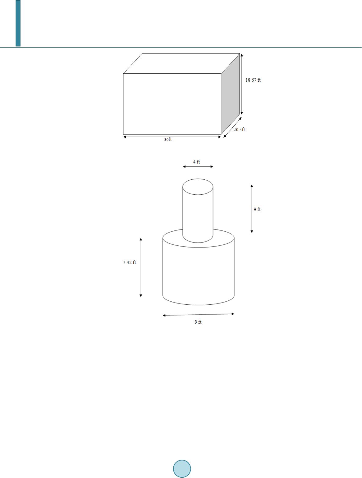 M. Mudragaddam et al. Figure 1. Schematic diagram of a wet well (Site 1). Figure 2. Schematic diagram of a wet well (Site 2). puter for reporting, analyzing and archiving. The best thing about this instrument is the data logging function which it has. The time interval between the readings can be set in the instrument, and the instrument will take the readings by turning on and off itself to the time interval specified. This instrument measures CO2 in percent (%) which has to be converted to parts per million by multiplying the percentage with 104. The H2S readings are measured directly in ppm by the instrument. The range of CO2 and H2S for this instrument are 0% - 100% and 0 - 500 ppm respectively. 4. Methods to Control H2S Emissions Wastewater Listed below are few methods available to control the rate of hydrogen sulfide corrosion. 1) Reducing the dissolved sulfide content of the wastewater 2) Using corrosion-resistant materials and coatings 3) Providing ventilation of the enclosed area of the sewer and 4) Conducting routine preventive maintenance.  M. Mudragaddam et al. Three basic techniques to control dissolved sulfide: a) Oxidation by the addition of chemical oxidants such as hydrogen peroxide, chlorine or potassium perman- ganate, or by the introduction of air or oxygen. b) Precipitation of dissolved sulfide by the addition of metallic salts such as ferrous chloride and ferrous sul- fate. c) pH elevation through the addition of sodium hydroxide. Since low pH is favorable to produce H2S gas, so it has to be increased (EPA, 1991). 5. Methodology Wastewater during its stay in a wet well produces CO2 and H2S gas. When the volume of wastewater increases in the well these gases are expelled out. Landtec GEM-2000 Plus, a CO2 and H2S detecting instrument is used to measure these gases inside the wet well. This instrument gives the concentration of CO2 in percentage and H2S in ppm (parts per million). The percentage measure is converted into ppm by multiplying it by 104 (0.1% = 1000 ppm). One ppm here means one part of CO2 or H2S is present in one million parts of air. As the volume of the wastewater in the wet well increases, these gases are pushed out, when the volume of wastewater decreases the surrounding ambient air is dragged into the well to fill the water column with the air. Hence the concentrations in the air volume of the wet well changes depending upon the water level in the well. Steps for Calculation: CO2 and H2S emissions from the wet well in terms of pounds can be calculated as below: CO2 expelled out of the wet well (lb) = Volume of Air Expelled Due to Increase in the water level *Average Hourly Concentration of CO2/H2S in the Wet Well * CO2/H2S density Assuming CO2 density at standard temperature and pressure = 1.98 kg/m 3 = 0.124 lb/ft3 The density of H2S is 1.363 kg/m3 equal to 0.085 1 lb /ft 3. CO2 and H2S emissions from the wet well in terms of pounds per cubic feet can be calculated as below: CO2 or H2S emitted per unit volume of wastewater (lb/ft3) = mass of CO2 or H2S emitted/average hourly volume of wastewater present in the wet well = mass of CO2 or H2S/[(V1 + V2)/2] where V1 = Initial volume of wastewater present in the wet well V2 = Final volume of wastewater present in the wet well. If a person takes a gas (CO2 or H2S) measurement at 8 A.M. and another gas measurement at 9 A.M., the Volume of wastewater present in the wet well at 8 A.M. is considered as the initial volume of wastewater and the volume of wastewater present in the wet well at 9 A.M. is considered as the final volume of the wastewater. If that person takes another gas measurement at 10 A.M., for the next calculation the volume of wastewater pre- sent in the wet well at 9 A.M. will become initial volume of wastewater present in the wet well and the volume of wastewater present in the wet well at 10 A.M. will be the final volume of wastewater present in the well. 5.1. Tables and Calculations Below calculations are made assuming the wet well is closed, and anaerobic conditions exist within the well. The measurements of the concentrations were taken on dry and hot day. Sample calculation for Table 1: Column 1: Time at which the CO2 reading is taken Column 2: Wastewater level in the wet well at the time of reading = 3.3 ft Dimensions of the wet well: Length = 36 ft Width = 20.5 ft Depth = 18.67 ft Column 3: Volume of wastewater present in the wet well = Length * Width* Wastewater level in the wet well = 36ft * 20.5ft * 3.3ft = 2435.4 ft3  M. Mudragaddam et al. Total volume of the wet well = Length * Width * Total Depth = 36ft *20.5 ft *18.67ft = 13778.46 ft3 Column 4: Volume of Air in the wet well = Total Volume of the wet well – Volume of water in the wet well = 13778.46 ft3 – 2435.4 ft3 = 11343.06 ft3 Column 5: Volume of Air expelled out due to increase in the water level = Difference between two consecutive air volumes = 11343.06 ft3 – 10752.66 ft3 = 590.4 ft3 Column 6: Concentration of CO2 in the Air in the Wet Well (ppm) = 3000 ppm, CO2 reading in the Landtec GEM-2000 Plus instrument inside the wet well Column 7: Average hourly concentration of CO2 in the wet well = Sum of two consecutive readings/2 = (3000 ppm +1000 ppm)/2 = 2000 ppm Column 8: Assuming CO2 density at standard temperature and pressure = 1.98 kg/m3 = 0.124 lb/ft3 CO2 expelled out of the wet well (lb) = Volume of Air Expelled Due to Increase in the water level * Average Hourly Concentration of CO2 in the Wet Well * CO2 dens i ty = 590.4 ft3 * 2000 ppm *0.124 lb/ft3 = 590.4 ft3 * 2000 ft3/ft3 *10-6 * 0.124 lb/ft3 = 0.146 lb Column 9: Average Hourly Volume of Water present in the Wet Well (ft3) = (2435.4 ft3 + 3025.8 ft3)/2 = 2730.6 ft3 Column 10: CO2 Emitted per unit volume of waste water (lb/ft3) = (CO2 e xpe lled out of the wet well (lb)/Average Hourly Volume of Water present in the Wet Well (ft3)) = 0.146 lb/2730.6 ft3 = 5.3622E-05 lb/ ft3 Every hour 0.146 pounds of CO2is emitted out of the wet well. For one cubic feet of wastewater 5.3622E-05 lb of CO2 is emitted. Similarly CO2 expelled out for the other wet well and H2S expelled out for the same wet well are calculated. The density of H2S is 1.363 kg/m3 equal to 0.0851 lb/ft3. For the Wet Well #2 lift station the H2S emissions could not be detected as the emissions were lower than the least count of the instrument. 6. Health Impacts 6.1. Health effects of CO2 Exposure to CO2 can produce a variety of health effects. These may include headaches, dizziness, restlessness, a tingling or pins or needles feeling, difficulty breathing, sweating, tiredness, increased heart rate, elevated blood pressure, coma, asphyxia to convulsions and even frostbite if exposed to dry ice. The levels of CO2 in the air and potential health problems are:  M. Mudragaddam et al. 1) 250 - 350 ppm—background (normal) outdoor air level. 2) 350 - 1000 ppm—typical level found in occupied spaces with good air exchange. 3) 1000 - 2000 ppm—level associated with complaints of drowsiness and poor air. 4) 2000 - 5000 ppm—level associated with headaches, sleepiness, and stagnant, stale, stuffy air. Poor concen- tration, loss of attention, increased heart rate and slight nausea may also be present. 5) >5000 ppm—Exposure may lead to severe oxygen deprivation resulting in permanent brain damage, coma and even death. Also, CO2 in the atmosphere increases the Earth’s temperature which is known as “green house effect” (US Department of Health Education and Welfare, Public Health Service, Centre for Disease Control, National Insti- tute for Occupational Safety and Health, 1976). 6.2. Health effects of H2S The levels of H2S in the air and potential health problems are: 1) 0.13 ppm—This is the odor threshold. Odor is unpleasant. 2) 4.6 ppm—Strong, intense odor, but tolerable. Prolonged exposure may deaden the sense of smell. 3) 10 - 20 ppm—Causes painful eyes, nose and throat irritation, headaches, fatigue, irritability, insomnia, gas- trointestinal disturbance, loss of appetite, dizziness. Prolonged exposure may cause bronchitis and pneumonia. 4) 50 ppm—May cause muscle fatigue, inflammation and dryness of nose, throat and tubes leading to the lungs. Exposure for one hour or more at levels above 50 ppm can cause severe eye tissue damage. Long-term exposure can cause lung disease. 5) 100 - 150 ppm—Loss of smell, stinging of eyes and throat. Fatal after 8 to 48 hours of continuous exposure. 6) 200 - 250 ppm—Nervous system depression (headache, dizziness and nausea are symptoms). Prolonged exposure may cause fluid accumulation in the lungs. Fatal in 4 to 8 hours of continuous exposure. 7) 250 - 600 ppm—Pulmonary edema (lungs fill with fluid, foaming in the mouth, chemical damage to lungs). 8) 300 ppm—May cause muscle cramps, low blood pressure and unconsciousness after 20 minutes. 9) 300 to 500 ppm may be fatal in 1 to 4 hours of continuous exposure. 10) 500 ppm—Paralyzes the respiratory system and overcomes victim almost instantaneously. Death after exposure of 30 to 60 minutes. 11) 700—Paralysis of the nervous system. 12) 1000—Immediately fatal. If caught in time, poisoning can be treated, and its effects are reversible. Some workers may experience ab- normal reflexes-dizziness, insomnia and loss of appetite that lasts for months or years. Acute poisoning does not result in death, may produce long-term symptoms such as loss of memory or depression, paralysis of facial mus- cles (Canadian Centre for Occupational Health and Safety, 1985). 7. Results and Discussion At Wet Well # 1 On an average CO2 expelled out of the wet well every one hour = 0.139 lb On an average H2S expelled out of the wet well every one hour = 0.002 lb CO2 emitted per unit volume of wastewater (lb/ft3) = 4.3715E-05 lb/ft3 H2S emitted per unit volume of wastewater (lb/ft3) = 6.7177E-07 lb/ft3 At Wet Well #2 On an average CO2 expelled out of the wet well every one hour = 0.002 lb CO2 emitted per unit volume of wastewater (lb/ft3) = 2.2545E-05 lb/ft3 It can be observed from Tabl es 1-3 that the concentrations of pollutants in the well change with temperature, size of the well, and volume of water present in the wet well. The concentrations of the pollutants also depend upon whether the wet well is directly exposed to the atmosphere or a superstructure exists above it. If a super- structure exists over a wet well, the conditions in the wet well may be considered as strictly anaerobic. Temper- ature is a very significant component for the H2S emissions, higher the temperature greater the gas emitted. CO2 emissions are less dependent on temperature when compared to H2S emissions. According to EPA, even at very low concentration (<1 ppm) of hydrogen sulfide, it can corrode the electrical and mechanical devices and also the concrete structures. The observed lift station exhibits higher hydrogen sulfide levels posing corrosion risks to  M. Mudragaddam et al. Table 1. CO2 emissions from the wet well. LIFT STATION: Wet Well # 1 Time (1) (Date: 06/12/09) Dry Weather (ft) (2) Volume of WW in the Wet Well (ft3) (3) Volume of Air in the Wet Well (ft3) (Total Volume of the wet well = 13778.46 ft3) (4) Volume of Due to Increase in water level (ft3) (5) of CO2 in the Air in the Wet Well (ppm) (6) Average Hourly Concentration of CO2 in the Wet Well (ppm) (7) 2 Well (lb) (8 ) Average Hourly Volume of WW present in the Wet Well (ft3) (9) CO2 per unit vo- (lb/ft3) ( 10) 10.00 AM 3.3 2435.4 11343.06 - 3000.0 - - - - 11.00 AM 4.1 3025.8 10752.66 590.4 1000.0 2000.0 0.146 2730.6 5.3622E-05 12 NOON 5.2 3 837.6 9940.86 811.8 4000.0 2500.0 0.252 3431.7 7.3333E-05 1.00 PM 3.6 2 656.8 1112 1. 66 0.0 3000.0 3500 .0 0.000 3247.2 0 2.00 PM 5.5 4 059.0 9719.46 1402.2 2 000.0 2500 .0 0.435 3357.9 0.0001 2945 3.00 PM 4.6 3 394.8 1038 3. 66 0.0 0.0 1000 .0 0.000 3726.9 0 4.00PM 3.0 2 214.0 1156 4. 46 0.0 1000.0 500.0 0.000 2804.4 0 5.00 PM 4.5 3 321.0 1045 7. 46 1107.0 1 000.0 1000.0 0.137 2767.5 0.0000 496 Average CO2 Expelled out of the Wet Well per one hour = 0.139 CO2 emitted/unit volume of WW = 4.3715E-05 Table 2. H2S emissions from the wet well. LIFT STATION: Wet Well # 1 Time (1) (Date: 06/12/09) Dry Weather Time (ft) Volume of WW in the Wet Well (ft3) Volume of Air (ft3) (Total Volume of the wet well = 13778.46 ft3) Volume of Air Expelled Due to Increase in 3 of H2S in the Well (ppm) Average Hourly Concentration of H2S in the Wet Well (ppm) H2 out of the Average Hourly Volume of WW present in the Wet Well (ft3) H2S Emi per unit volume of WW (lb/ft3) 10.00 AM 3.3 2435.4 1134 3.06 - 19.0 - - - - 11.00 AM 4.1 3025.8 1075 2.66 590.4 6.0 12.5 0.001 2730.6 0.00000023 12 NOON 5.2 3837.6 9940.86 811.8 69.0 37.5 0.003 3431.7 7.5492E-07 1.00 PM 3.6 2656.8 11121.66 0.0 89. 0 79. 0 0.000 3247.2 0 2.00 PM 5.5 4059.0 9719.46 1402.2 57.0 73. 0 0.009 3357.9 2.5941E-06 3.00 PM 4.6 3394.8 10383.66 0.0 2.0 29.5 0.000 3726.9 0 4.00 PM 3.0 2214.0 11564.46 0.0 26. 0 14. 0 0.000 2804.4 0 5.00 PM 4.5 3321.0 10457.46 1 107.0 40.0 33. 0 0.003 2767.5 1.1233E-06 Average H2 S Expelled out of the Wet Well per one hour = 0.002 H2S emitted/unit volume of WW = 6.7177E-07  M. Mudragaddam et al. Table 3. CO2 emissions from the wet well. LIFT STATION: Wet Well # 2 Time (1) (Date: 06/12/09) Dry Weather Time WW Level in the Well (ft) Volume of WW in the (ft3) Volume of Air in the Wet Well (ft3) (Total Volume of the wet well = 585.1 ft3) Volume of Due to Increase in water level (ft3) Concentration of CO2 in the Air in the Wet Well (ppm) Average Hourly Concentration of CO2 in the Wet Well (ppm) CO2 Expelled out of the Wet Well (lb) Average Hourly Volume of WW present in the Wet Well (ft3) CO2 per unit volume of WW (lb/ft3) 9.30 AM 1.2 76.3 508.8 - 3000 - - - - 10.30 AM 2.1 133.6 451.5 57.3 1000 2000 0.014 104.96871 0.00013527 11.30 AM 2.3 146.3 438.8 12.7 1000 1000 0.002 139.95828 1.1273E-05 12.30 PM 2.0 127.2 457.9 0.0 0 500 0.000 136.77 741 0 1.30 PM 1.5 95.4 489.7 0.0 1000 500 0.000 111.33045 0 2.30 PM 1.8 114.5 470.6 19.1 0 500 0.001 104.96 871 1.1273E-05 3.30 PM 2.3 146.3 438.8 31.8 0 0 0.000 130.41567 0 4.30 PM 1.4 89.1 496.1 0.0 0 0 0.000 117.69219 0 Average CO2 Expelled out of the Wet Well per one hour = 0.002 CO2 emitted/unit volume of WW = 2.2545E-05 the Kenner City’s wastewater infrastructure. 8. Limita t ions Practically no wet well is completely closed. There may be some leakages from the well which are not considered in this approach of quantifying emissions. The emissions may change depending upon the composition of the wastewater, pH, temperature, and residence time inside the wet well which should be further investigated. References American Public Health Association, American Water Works Association, Water Environment Federation (19 95 ). Standard Metho ds for the Examination of Water and Wastewater (19th ed.). Washington DC: APH A. Canadian Centre for Occupational Health and Safety (1985). Chemical Hazard Summary: Hydrogen Sulfide No. 12. Hamil - ton: Canadian Centre for Occupational Health and Safety. El-Fadel, M., & M assoud, M. (200 1 ). Methane Emissions from Wastewater Management. Environmental Pollution, 114. Gerardi Michael, H, & Zimmerman Mel, C. (2005 ). Wastewater Pathogens. Hoboken: John Wiley & Sons, Inc. IPCC (20 01). Climate Change 2001: Synthesis Report. A Contribution of Working Groups I, II, and III to the Third Assess- ment Report of the Intergovernmental Panel on Climate Change (398 p). In Watson, R.T., & the Core Writing Team (Eds.), Cambridge, United Kingdom, and New York: Cambridge University Press. Metcalf, & Eddy Inc. (1991). Wastewater Engineering: Treatment, Disposal, and Reuse (3rd ed.). In G. Tchobanoglous, & F. L. Burton (Eds.), New York: M cGr aw -Hill. National Institute for Occupational Safety and Health/Occupational Safety and Health Administration (1981) NIOSH/OSHA: Occupational Health Guidelines for Chemical Hazards. Palmer, T., Lagasse, P., & Ross, M. (20 00 ). Hydrogen Sulfide Control in Wastewater Collection systems. Water Engineering and Management, 27-29. US Department of Health Education and Welfare, Public Health Service, Centre for disease control, National Institute for Occupational Safety and Health (1976). Occupational Exposure to Carbon Dioxide (pp. 76-194 ). NIOSH. US Department of Health Education and Welfare, Public Health Service, National Institute for Occupational Safety and  M. Mudragaddam et al. Health, Cincinnati. A Recommended Standard for Occupational Exposure to Hydrogen Sulfide. US Environmental Protection Agency (1991). Hydrogen Sulfide Corrosion: Its Consequences, Detection and Control. Vaughan Harshman, P. E., & Barnette, T. (2000). Wastewater Odor Control: An Evaluation of Technologies.
|