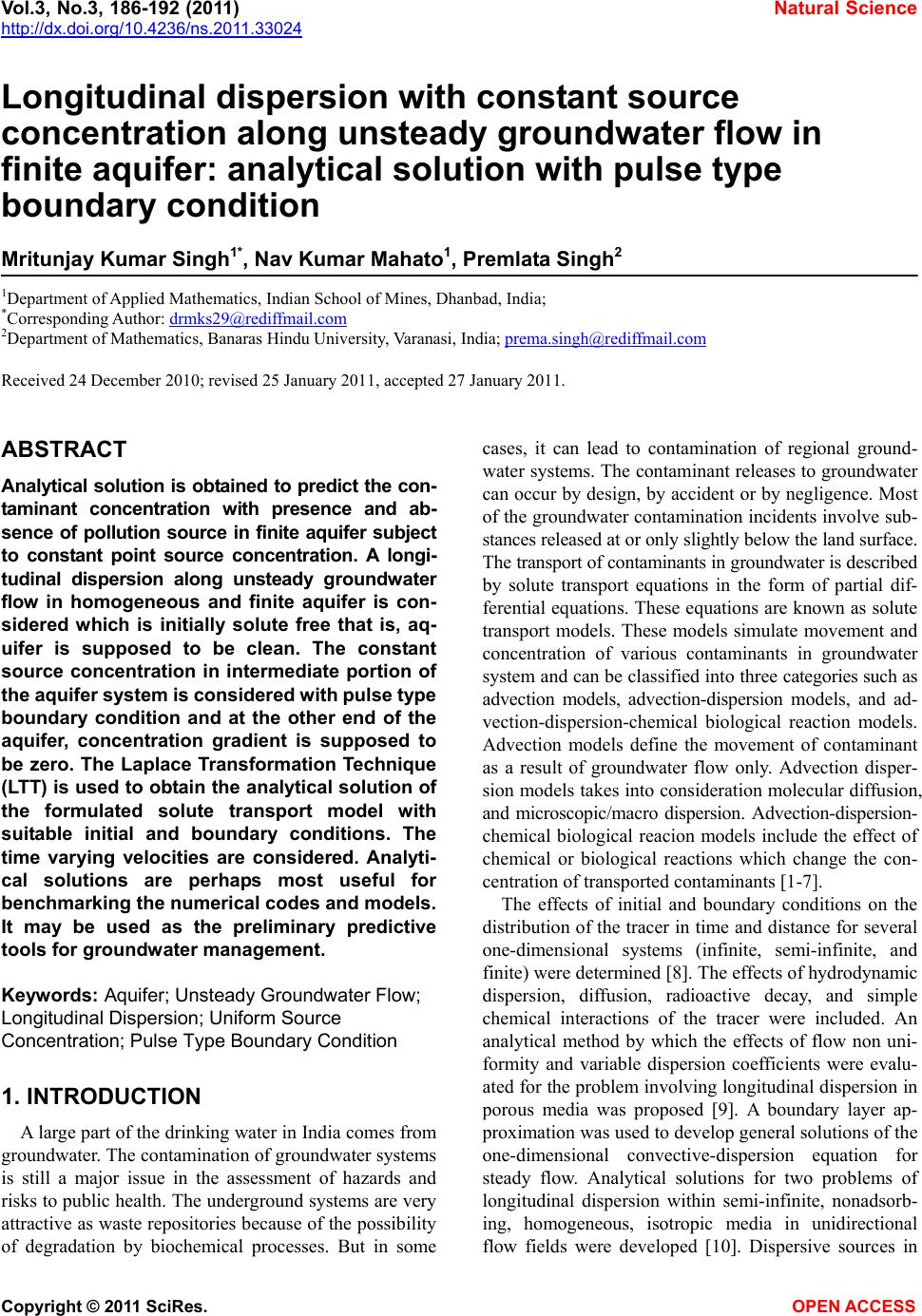
Vol.3, No.3, 186-192 (2011) Natural Science
http://dx.doi.org/10.4236/ns.2011.33024
Longitudinal dispersion with constant source
concentration along unsteady groundwater flow in
finite aquifer: analytical solution with pulse type
boundary condition
Mritunjay Kumar Singh1*, Nav Kumar Mahato1, Premlata Singh2
1Department of Applied Mathematics, Indian School of Mines, Dhanbad, India;
*Corresponding Author:
2Department of Mathematics, Banaras Hindu University, Varanasi, India;
Received 24 December 2010; revised 25 January 2011, accepted 27 January 2011.
ABSTRACT
Analytical solution is obtained to predict the con-
taminant concentration with presence and ab-
sence of pollution source in finite aquifer subject
to constant point source concentration. A longi-
tudinal dispersion along unsteady groundwater
flow in homogeneous and finite aquifer is con-
sidered which is initially solute free that is, aq-
uifer is supposed to be clean. The constant
source concentration in intermediate portion of
the aquifer system is considered with pulse type
boundary condition and at the other end of the
aquifer, concentration gradient is supposed to
be zero. The Laplace Transformation Technique
(LTT) is used to obtain the analytical solution of
the formulated solute transport model with
suitable initial and boundary conditions. The
time varying velocities are considered. Analyti-
cal solutions are perhaps most useful for
benchmarking the numerical codes and models.
It may be used as the preliminary predictive
tools for groundwater management.
Keywords: Aquifer; Unsteady Groundwater Flow;
Longitudinal Dispersion; Uniform Source
Concentration; Pulse Type Boundary Condition
1. INTRODUCTION
A large part of the drinking water in India comes from
groundwater. The contamination of groundwater systems
is still a major issue in the assessment of hazards and
risks to public health. The underground systems are very
attractive as waste repositories because of the possibility
of degradation by biochemical processes. But in some
cases, it can lead to contamination of regional ground-
water systems. The contaminant releases to groundwater
can occur by design, by accident or by negligence. Most
of the groundwater contamination incidents involve sub-
stances released at or only slightly below the land surface.
The transport of contaminants in groundwater is described
by solute transport equations in the form of partial dif-
ferential equations. These equations are known as solute
transport models. These models simulate movement and
concentration of various contaminants in groundwater
system and can be classified into three categories such as
advection models, advection-dispersion models, and ad-
vection-dispersion-chemical biological reaction models.
Advection models define the movement of contaminant
as a result of groundwater flow only. Advection disper-
sion models takes into consideration molecular diffusion,
and microscopic/macro dispersion. Advection-dispersion-
chemical biological reacion models include the effect of
chemical or biological reactions which change the con-
centration of transported contaminants [1-7].
The effects of initial and boundary conditions on the
distribution of the tracer in time and distance for several
one-dimensional systems (infinite, semi-infinite, and
finite) were determined [8]. The effects of hydrodynamic
dispersion, diffusion, radioactive decay, and simple
chemical interactions of the tracer were included. An
analytical method by which the effects of flow non uni-
formity and variable dispersion coefficients were evalu-
ated for the problem involving longitudinal dispersion in
porous media was proposed [9]. A boundary layer ap-
proximation was used to develop general solutions of the
one-dimensional convective-dispersion equation for
steady flow. Analytical solutions for two problems of
longitudinal dispersion within semi-infinite, nonadsorb-
ing, homogeneous, isotropic media in unidirectional
flow fields were developed [10]. Dispersive sources in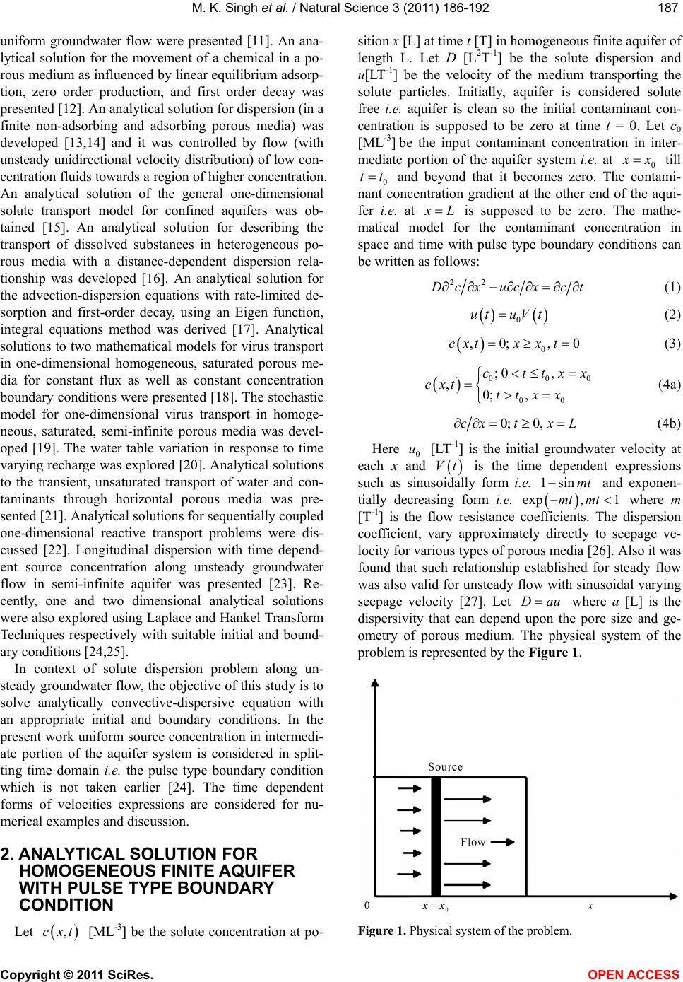

M. K. Singh et al. / Natural Science 3 (2011) 186-192
187187
uniform groundwater flow were presented [11]. An ana-
lytical solution for the movement of a chemical in a po-
rous medium as influenced by linear equilibrium adsorp-
tion, zero order production, and first order decay was
presented [12]. An analytical solution for dispersion (in a
finite non-adsorbing and adsorbing porous media) was
developed [13,14] and it was controlled by flow (with
unsteady unidirectional velocity distribution) of low con-
centration fluids towards a region of higher concentration.
An analytical solution of the general one-dimensional
solute transport model for confined aquifers was ob-
tained [15]. An analytical solution for describing the
transport of dissolved substances in heterogeneous po-
rous media with a distance-dependent dispersion rela-
tionship was developed [16]. An analytical solution for
the advection-dispersion equations with rate-limited de-
sorption and first-order decay, using an Eigen function,
integral equations method was derived [17]. Analytical
solutions to two mathematical models for virus transport
in one-dimensional homogeneous, saturated porous me-
dia for constant flux as well as constant concentration
boundary conditions were presented [18]. The stochastic
model for one-dimensional virus transport in homoge-
neous, saturated, semi-infinite porous media was devel-
oped [19]. The water table variation in response to time
varying recharge was explored [20]. Analytical solutions
to the transient, unsaturated transport of water and con-
taminants through horizontal porous media was pre-
sented [21]. Analytical solutions for sequentially coupled
one-dimensional reactive transport problems were dis-
cussed [22]. Longitudinal dispersion with time depend-
ent source concentration along unsteady groundwater
flow in semi-infinite aquifer was presented [23]. Re-
cently, one and two dimensional analytical solutions
were also explored using Laplace and Hankel Transform
Techniques respectively with suitable initial and bound-
ary conditions [24,25].
In context of solute dispersion problem along un-
steady groundwater flow, the objective of this study is to
solve analytically convective-dispersive equation with
an appropriate initial and boundary conditions. In the
present work uniform source concentration in intermedi-
ate portion of the aquifer system is considered in split-
ting time domain i.e. the pulse type boundary condition
which is not taken earlier [24]. The time dependent
forms of velocities expressions are considered for nu-
merical examples and discussion.
2. ANALYTICAL SOLUTION FOR
HOMOGENEOUS FINITE AQUIFER
WITH PULSE TYPE BOUNDARY
CONDITION
Let

,cxt [ML-3] be the solute concentration at po-
sition x [L] at time t [T] in homogeneous finite aquifer of
length L. Let D [L2T-1] be the solute dispersion and
u[LT-1] be the velocity of the medium transporting the
solute particles. Initially, aquifer is considered solute
free i.e. aquifer is clean so the initial contaminant con-
centration is supposed to be zero at time t = 0. Let c0
[ML-3] be the input contaminant concentration in inter-
mediate portion of the aquifer system i.e. at 0
x
x

till
0
tt

and beyond that it becomes zero. The contami-
nant concentration gradient at the other end of the aqui-
fer i.e. at
x
L

is supposed to be zero. The mathe-
matical model for the contaminant concentration in
space and time with pulse type boundary conditions can
be written as follows:
22
Dcx ucxct

 (1)


0
ut uVt (2)


0
,0; ,0cxtxx t

 (3)

000
00
;0 ,
,0; ,
cttxx
cxt ttxx




 (4a)
0; 0,cxtx L

 (4b)
Here 0 u [LT-1] is the initial groundwater velocity at
each x and


Vt is the time dependent expressions
such as sinusoidally form i.e. 1sinmt and exponen-
tially decreasing form i.e.

exp, 1mt mt where m
[T-1] is the flow resistance coefficients. The dispersion
coefficient, vary approximately directly to seepage ve-
locity for various types of porous media [26]. Also it was
found that such relationship established for steady flow
was also valid for unsteady flow with sinusoidal varying
seepage velocity [27]. Let Dau where a [L] is the
dispersivity that can depend upon the pore size and ge-
ometry of porous medium. The physical system of the
problem is represented by the Figure 1.
Figure 1. Physical system of the problem.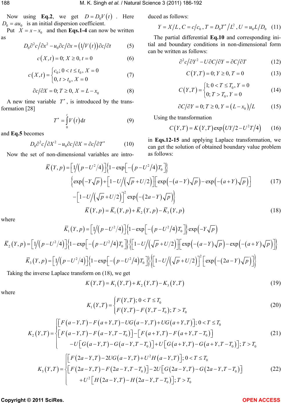

M. K. Singh et al. / Natural Science 3 (2011) 186-192 188
Now using Eq.2, we get

0
DDVt. Here
00
Dau is an initial dispersion coefficient.
Put 0
X
xx and then Eqs.1-4 can now be written
as
 
22
00
1Dcx ucxVtct 
(5)

,0; 0,0cXtX t (6)

00
0
;0, 0
,0,, 0
cttX
cXt ttX
 


 (7)
0
0; 0,cXTX Lx   (8)
A new time variable T, is introduced by the trans-
formation [28]

0
d
t
TVtt
 (9)
and Eq.5 becomes
22
00
DcX ucXcT

 (10)
Now the set of non-dimensional variables are intro-
duced as follows:
2
00 00
,, ,YXLCccTDTLUuLD

 (11)
The partial differential Eq.10 and corresponding ini-
tial and boundary conditions in non-dimensional form
can be written as follows:
22
cY UCYCT

 (12)


,0;0,0CYTY T

 (13)

0
0
1; 0,0
,0;, 0
TTY
CYT TTY
 


 (14)

0
0; 0,CYTYLx L (15)
Using the transformation





2
,,exp24CYTKYTUYUT (16)
in Eqs.12-15 and applying Laplace transformation, we
can get the solution of obtained boundary value problem
as follows:






 









22
0
2
,1 41exp4
exp12 expexp
12exp2
KYppUp UT
YpUpUaYpaY p
UpU aYp
 
 
 
 
 
 

 

(17)







123
,,,,
K
YpK YpKYpKYp (18)
where








22
10
,141 exp4exp
K
YppUpUTY p
 
 


 











22
20
,141 exp412expexpKYppUpUTUpUaY paY p

 
 
 
 



 







2
22
30
,141 exp412exp2KYppUpUTUpUaY p

 
 
 
 

 
Taking the inverse Laplace transform on (18), we get







123
,,,,
K
YTK YTKYTKYT (19)
where



 
0
1
00
,;0
,,,;
FYTT T
KYT
F
YTFYTTTT







(20)






   
0
200
000
,, , ,;0
,,, ,,
,, ,,;
FaYTF aYTUG aYTUG aYTTT
KYTFaYT FaYTTFaYT FaYTT
UGaYT GaYTTUGaYT GaYTTTT
  








 


(21)








2
0
300
2
00
2,2 ,,;0
,2,2,2 2,2,
2, 2, ;
Fa YTUGa YTUHa YTTT
K
YTFa YTFa YTTUGaYTGa YTT
U H aYTH aYTTTT

 



 





(22)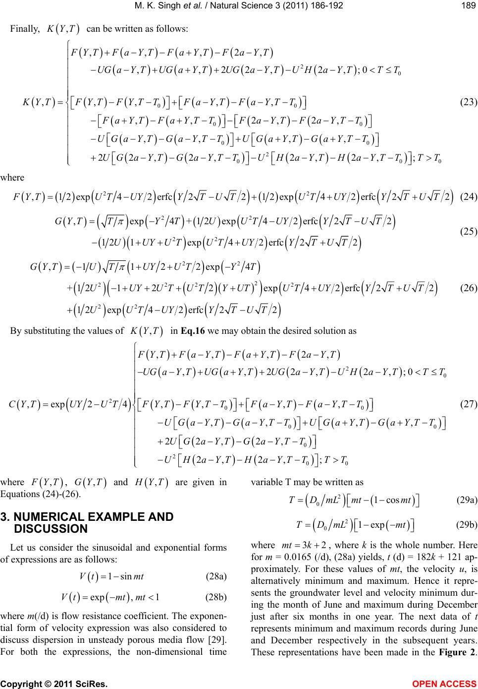

M. K. Singh et al. / Natural Science 3 (2011) 186-192
189189
Finally,

,
K
YT can be written as follows:

  

   
   




2
0
00
00
00
,,,2,
,,22,2,;0
,,,, ,
,,2,2,
,, ,,
FYTFaYTFaYTFaYT
UGaY TUGaY TUGaYTUHaY TTT
K YTF YTFYTTFaYTF aYTT
Fa YTFa YTTFa YTFa YTT
UGaYT GaYTTUGaYT GaYTT
  

  
 

 

 


   
2
000
22, 2,2,2,;UG aYTG aYTTUHaYTHaYTTT T












 
 
 

(23)
where

 


 
2 2
,12 exp42 erfc2212 exp42 erfc22FYT UTUYYTUTUTUYYTUT  (24)









 
22
22
,exp4+12exp42erfc22
121exp42 erfc22
GYTTYTUUTUYYTU T
UUYUT UTUYYTUT
  
  (25)




 




 
22
2
222 2
22
,1 122exp4
+1 2122exp42erfc22
1 2exp42erfc22
GYTUTUYUTYT
UUYUTUTYUTU TUYYTUT
UUTUY YTUT
  
 

(26)
By substituting the values of

,
K
YT in Eq.16 we may obtain the desired solution as


 





   
 
2
0
2
00
00
0
2
,,,2,
,,22,2,;0
,exp 24,,,,
,, ,,
22, 2,
2,
FYTFaYTFaYTFaYT
UGaY TUGaY TUGaY TUHaY TTT
CYTUYUTFYTFYTTFaYTFaYTT
UGaYT GaYTTUGaYT GaYTT
UG aYTG aYTT
UHaY
  
 
   
 
 

 


 
00
2, ;THaYTT TT













 


(27)
where


,
F
YT ,


,GYT and

,
H
YT are given in
Equations (24)-(26).
3. NUMERICAL EXAMPLE AND
DISCUSSION
Let us consider the sinusoidal and exponential forms
of expressions are as follows:

1sinVtmt (28a)
 
exp, 1V tmtmt  (28b)
where m(/d) is flow resistance coefficient. The exponen-
tial form of velocity expression was also considered to
discuss dispersion in unsteady porous media flow [29].
For both the expressions, the non-dimensional time
variable T may be written as



2
01cosTD mLmtmt



 (29a)



2
01expTD mLmt



 (29b)
where 32mt k

, where k is the whole number. Here
for m = 0.0165 (/d), (28a) yields, t (d) = 182k + 121 ap-
proximately. For these values of mt, the velocity u, is
alternatively minimum and maximum. Hence it repre-
sents the groundwater level and velocity minimum dur-
ing the month of June and maximum during December
just after six months in one year. The next data of t
represents minimum and maximum records during June
and December respectively in the subsequent years.
These representations have been made in the Figure 2.

M. K. Singh et al. / Natural Science 3 (2011) 186-192 190
Figure 2. Time dependent sinusoidal form of velocity represen-
tations.
Analytical solutions (27) is solved for the values 01.0c

,
00.001u km/d, 01.0D km2/d, and L = 100 km.
The concentration values in the presence of source pol-
lution till 0
tt (1500 d) are depicted graphically in the
presence of constant source of contaminants at
32mt k, where 27k which represents mini-
mum and maximum records of groundwater level and
velocity during June and December in 2nd, 3rd and 4th
years at the respective time values t (d). When the source
is eliminated the solution is solved at 32mt k

,
where 813k which represent the duration of June
and December alternatively in the 5th, 6th and 7th years
respectively. The contaminants concentration distribu-
tion behaviour along unsteady flow of sinusoidal form of
velocity given in (28a) depicted in the Figure 3(a) when
0
TT and Figure 3(b) when 0 TT. It is observed
that the contaminant concentration decreases with time
and distance traveled in presence of source contaminants.
While in the absence of source contaminants, it increases
and goes on increasing which attains towards maximum
and then starts decreases and goes on decreasing which
attains towards minimum or harmless concentration.
This decreasing tendency of contaminant concentration
with time and distance traveled may help to rehabilitate
the contaminated aquifer. For the same set of inputs ex-
cept m = 0.0002 (/d) as 1mt , Eq.27 is also computed
for exponentially decreasing form of velocity given in
(28b). It is observed that the contaminant concentration
follows almost the same trend in presence and absence
of source contaminants respectively. This decreasing
tendency of contaminant concentration with time and
distance traveled is depicted graphically in Figure 4(a)
when 0
TT and Figure 4(b) if 0 TT for exponen-
tially decreasing form of velocity.
(a)
(b)
Figure 3. Contaminants concentration along unsteady ground-
water flow of sinusoidal form of velocity in homogeneous
finite aquifer when (a) T ≤ T0 and (b) T > T0.
4. CONCLUSIONS
A solute transport model is solved analytically with
constant source of input concentration in homogeneous
finite aquifer. The pulse type boundary conditions are
considered in intermediate portion of the aquifer system.
The time varying velocities are taken in to consideration
in which one such form i.e. sinusoidal form represents
the seasonal variation in a year in tropical regions. The
Laplace Transform Technique is used to get an analytical
solution which is perhaps most useful for benchmarking
the numerical codes and models. The result of the prob-
lem may be used as the preliminary predictive tools for
groundwater management. The solution is obtained and

M. K. Singh et al. / Natural Science 3 (2011) 186-192
191191
(a)
(b)
Figure 4. Contaminants concentration along unsteady ground-
water flow of exponential form of velocity in homogeneous
finite aquifer when (a) T ≤ T0 and (b) T > T0.
graphical representations are made under the assumption
0
x
x which is the limitation of the solution of the
problem. The solution in the domain 0
x
x is not con-
sidered in the present work only because the solute con-
centration will not remain in this domain for the longer
period. After very short duration of time it will move on
in the domain 0
x
x [14].
5. ACKNOWLEDGEMENTS
The first author is grateful to the University Grants Commission,
New Delhi, and Government of India for their financial support to
carry out the research work. The authors are thankful to the reviewers
for their constructive comments.
REFERENCES
[1] Fried, J.J. (1975) Groundwater pollution. Elsevier Scien-
tific Publishing Company, Amsterdam.
[2] Ghosh Bobba, A. and Singh, V.P. (1995) Groundwater
contamination modeling. In: Singh, V.P., Ed., Envior-
mental hydrology, Kluwer Academic Publishers, Dord-
recht, 225-319.
[3] Charbeneau, R.J. (2000) Groundwater hydraulics and
pollutant transport. Prentice Hall, New Jersey.
[4] Rai, S.N. (2004) Role of mathematical modeling. In: Rai,
S. N., Ed., Groundwater Resource Management, NGRI,
Hyderabad.
[5] Sharma, H.D. and Reddy, K.R. (2004) Geo-environ-
mental Engineering. John Willy & Sons, INC.
[6] Rausch, R., Schafer, W., Therrien, R. and Wagner, C.
(2005) Solute transport modelling: An introduction to
models and solution strategies. Gebr. Borntrager Ver-
lagsbuchhandlung Science Publishers, Berlin.
[7] Thangarajan, M. (2006) Groundwater: Resource evalua-
tion, augmnetation, contamination, restoration, modeling
and management. Capital Publishing Company, New
Delhi, 362.
[8] Gershon, N.D. and Nir, A. (1969) Effects of boundary
conditions of models on tracer distribution in flow
through porous mediums. Water Resources Research, 5,
830-839. doi:10.1029/WR005i004p00830
[9] Gelher, L.W. and Collins, M.A. (1971) General analysis
of longitudinal dispersion in non-uniform flow. Water
Resources Research, 7, 1511-1521.
doi:10.1029/WR007i006p01511
[10] Marino, M.A. (1974) Longitudinal dispersion in satu-
rated porous media. Journal of the Hydraulics Division,
100, 151-157.
[11] Hunt, B. (1978) Dispersive sources in uniform ground
water flow. Journal of the Hydraulics Division, 104,
75-85.
[12] Van Genuchten, M.Th. (1981) Analytical solutions for
chemical transport with simultaneous adsorption, zero
order production and first order decay. Journal of Hy-
drology, 49, 213-233.
[13] Kumar, N. (1983) Unsteady flow against dispersion in
finite porous media. Journal of Hydrology, 63, 345-358.
doi:10.1016/0022-1694(83)90050-1
[14] Kumar, N. and Kumar, M. (1998) Solute dispersion along
unsteady groundwater flow in a semi-infinite aquifer;
Hydrology and Earth System Sciences, 2, 93-100.
doi:10.5194/hess-2-93-1998
[15] Lindstrom, F.T. and Boersma, L. (1989) Analytical solu-
tions for convective-dispersive transport in confined aq-
uifers with different initial and boundary conditions. Wa-
ter Resources Research, 25, 241-256.
doi:10.1029/WR025i002p00241
[16] Yates, S.R. (1990) An analytical solution for one-di-
mensional transport in heterogeneous porous media. Wa-
ter Resources Research, 26, 2331-2338.
doi:10.1029/WR026i010p02331
[17] Fry, V.A. and Istok, J.D. (1993) An analytical solution to
the solute transport equation with rate-limited desorption
and decay. Water Resources Research, 29, 3201-3208.
doi:10.1029/93WR01394

M. K. Singh et al. / Natural Science 3 (2011) 186-192 192
[18] Sim, Y. and Chrysikopoulos, C.V. (1995) Analytical
models for one-dimensional virus transport in saturated
porous media. Water Resources Research, 31, 1429-
1437. doi:10.1029/95WR00199
[19] Chrysikopoulos, C.V. and Sim, Y. (1996) One-dimen-
sional virus transport in homogeneous porous media with
time-dependent distribution coefficient. Journal of Hy-
drology, 185, 199-219.
[20] Rai, S.N. and Manglik, A. (1999) Modelling of water
table variation in response to time varying recharge from
multiple basin using the linearised Boussinesq equation.
Journal of Hydrology, 220, 141-148.
doi:10.1016/S0022-1694(99)00074-8
[21] Sander, G.C. and Braddock, R.D. (2005) Analytical solu-
tions to the transient, unsaturated transport of water and
contaminants through horizontal porous media. Advances
in Water Resources, 28, 1102-1111.
doi:10.1016/j.advwatres.2004.10.010
[22] Srinivasan, V., and Clement, T.P. (2008) Analytical solu-
tions for sequentially coupled one-dimensional reactive
transport problems-Part-I: Mathematical Derivations.
Advances in Water Resources, 31, 203.
doi:10.1016/j.advwatres.2007.08.002
[23] Singh, M.K., Mahato, N.K. and Singh, P. (2008) Longi-
tudinal dispersion with time dependent source concentra-
tion in semi infinite aquifer. Journal of Earth System
Science, 117, 945-949.
doi:10.1007/s12040-008-0079-x
[24] Singh, M.K., Singh, V.P., Singh, P., and Shukla, D. (2009)
Analytical solution for conservative solute transport in
one-dimensional homogeneous porous formations with
time dependent velocity. Journal of Engineering Me-
chanics, 135, 1015-1021.
doi:10.1061/(ASCE)EM.1943-7889.0000018
[25] Singh, M.K., Singh, P. and Singh, V.P. (2010) Two di-
mensional solute dispersion with time dependent source
concentration in finite aquifer. Journal of Engineering
Mechanics, 136, 1309-1315.
doi:10.1061/(ASCE)EM.1943-7889.0000177
[26] Ebach, E.H. and White, R. (1958) Mixing of fluid flow-
ing through beds of packed solids. Journal of American
Institute of Chemical Engineers, 4, 161-164.
[27] Rumer, R.R. (1962) Longitudinal dispersion in steady
and unsteady flow. Journal of the Hydraulics Division,
88, 147-172.
[28] Crank, J. (1975) The Mathematics of diffusion. Oxford
University Press, Oxford.
[29] Banks, R.B. and Jerasate, S. (1962) Dispersion in un-
steady porous media flow. Journal of the Hydraulics Di-
vision, 88, 1-21.