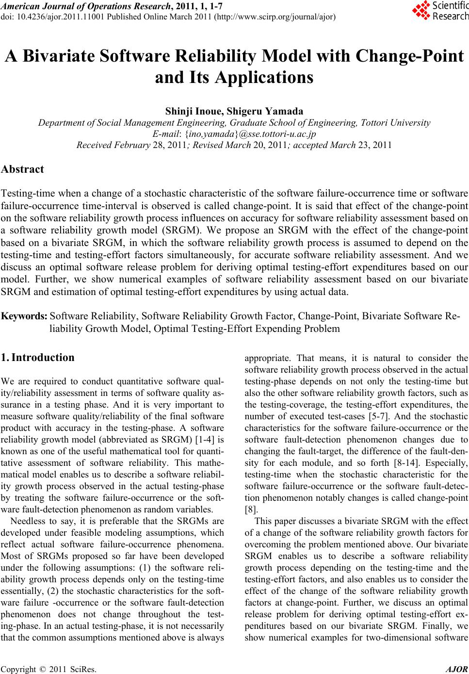
 American Journal of Operations Research, 2011, 1, 1-7 doi: 10.4236/ajor.2011.11001 Published Online March 2011 (http://www.scirp.org/journal/ajor) Copyright © 2011 SciRes. AJOR A Bivariate Software Reliability Model with Change-Point and Its Applications Shinji Inoue, Shigeru Yamada Department of Social Management Engineering, Graduate School of Engineering, Tottori University E-mail: {ino,yamada }@sse.tottori-u.ac.jp Received February 28, 2011; Revised March 20, 2011; accepted March 23, 2011 Abstract Testing-time when a change of a stochastic characteristic of the software failure-occurrence time or software failure-occurrence time-interval is observed is called change-point. It is said that effect of the change-point on the software reliability growth process influences on accuracy for software reliability assessment based on a software reliability growth model (SRGM). We propose an SRGM with the effect of the change-point based on a bivariate SRGM, in which the software reliability growth process is assumed to depend on the testing-time and testing-effort factors simultaneously, for accurate software reliability assessment. And we discuss an optimal software release problem for deriving optimal testing-effort expenditures based on our model. Further, we show numerical examples of software reliability assessment based on our bivariate SRGM and estimation of optimal testing-effort expenditures by using actual data. Keywords: Software Reliability, Software Reliability Growth Factor, Change-Point, Bivariate Software Re- liability Growth Model, Optimal Testing-Effort Expending Problem 1. Introduction We are required to conduct quantitative software qual- ity/reliability assessment in terms of software quality as- surance in a testing phase. And it is very important to measure software quality/reliability of the final software product with accuracy in the testing-phase. A software reliability growth model (abbreviated as SRGM) [1-4] is known as one of the useful mathematical tool for quanti- tative assessment of software reliability. This mathe- matical model enables us to describe a software reliabil- ity growth process observed in the actual testing-phase by treating the software failure-occurrence or the soft- ware fault-detection phenomenon as random variables. Needless to say, it is preferable that the SRGMs are developed under feasible modeling assumptions, which reflect actual software failure-occurrence phenomena. Most of SRGMs proposed so far have been developed under the following assumptions: (1) the software reli- ability growth process depends only on the testing-time essentially, (2) the stochastic characteristics for the soft- ware failure -occurrence or the software fault-detection phenomenon does not change throughout the test- ing-phase. In an actual testing-phase, it is not necessarily that the common assumptions mentioned above is always appropriate. That means, it is natural to consider the software reliability growth process observed in the actual testing-phase depends on not only the testing-time but also the other software reliability growth factors, such as the testing-coverage, the testing-effort expenditures, the number of executed test-cases [5-7]. And the stochastic characteristics for the software failure-occurrence or the software fault-detection phenomenon changes due to changing the fault-target, the difference of the fault-den- sity for each module, and so forth [8-14]. Especially, testing-time when the stochastic characteristic for the software failure-occurrence or the software fault-detec- tion phenomenon notably changes is called change-point [8]. This paper discusses a bivariate SRGM with the effect of a change of the software reliability growth factors for overcoming the problem mentioned above. Our bivariate SRGM enables us to describe a software reliability growth process depending on the testing-time and the testing-effort factors, and also enables us to consider the effect of the change of the software reliability growth factors at change-point. Further, we discuss an optimal release problem for deriving optimal testing-effort ex- penditures based on our bivariate SRGM. Finally, we show numerical examples for two-dimensional software  S. INOUE ET AL. 2 reliability analysis and estimation of an optimal test- ing-effort expenditures based on our bivariate model by using actual software fault data. 2. Two-Dimensional Software Reliability Growth Modeling A bivariate SRGM in which the number of detectable faults in a software system is assumed to be finite can be developed by the following modeling assumptions [5, 15,16]: (A1) Whenever a software failure is observed, the fault is detected immediately, and no new faults are intro- duced in the fault-detection procedures. (A2) Each software failure occurs at independently and identically distributed random times with the bivariate probability distribution function (, )Pr, suS sUu, where S and U are the ran dom variables representing the testing-time and cumulative testing-effort expenditure, respectively. And Pr represents the joint density function and the probability of event A, respectively. (A3) The initial number of faults in the software system, N0( > 0), is a random variable, and is finite. Figure 1 shows the stochastic quantities for the two- dimensional software failure-occurrence or the software fault-detection phenomenon. Now we define the two- dimensional stochastic process (, ),0,0Nsusu [17] representing the number of faults detected in the two-dimensional space [0,s] × [0,u]. Then, we have a bi- variate probability mass function that faults are de- tected in the two-dimensional space [0,s] × [0,u] as m 0 Pr ,,1, Pr (0,1,2,) mn n n NsumFsuFsu m Nn m m (1) from the modeling assumptions. From Equation. (1), we can say that the stochastic behavior of the software fail- ure-occurrence or the software fault-detection phenome- non can be characterized by assuming the probability mass function for the initial number of faults in the soft- ware system, N0. In this paper, we assume that the initial fault content follows a Poisson distribution with parame- ter ω. Then we have: (, ) Pr(, )exp(, ) ! m Fsu Nsu mFsu m (2) from Equation (1). Equation (2) is essentially equivalent to a two-dimensional nonhomogeneous Poisson process (abbreviated as a two-dimensional NHPP) [5,6] with Figure 1. Stochastic quantities for the two-dimensional software failure-occurrence of fault-detection phenomenon Figure 2. Two-dimensional stochastic quantities for the software failure-occurrence phenomenon with change –point mean value function , where ,(,)(,ENsusuFsu ) []E denotes the expectation. 3. Two-Dimensional Change -P oi nt Mo de li ng We discuss a bivariate software reliability growth model- ing with effect of change-point on the software reliability Copyright © 2011 SciRes. AJOR 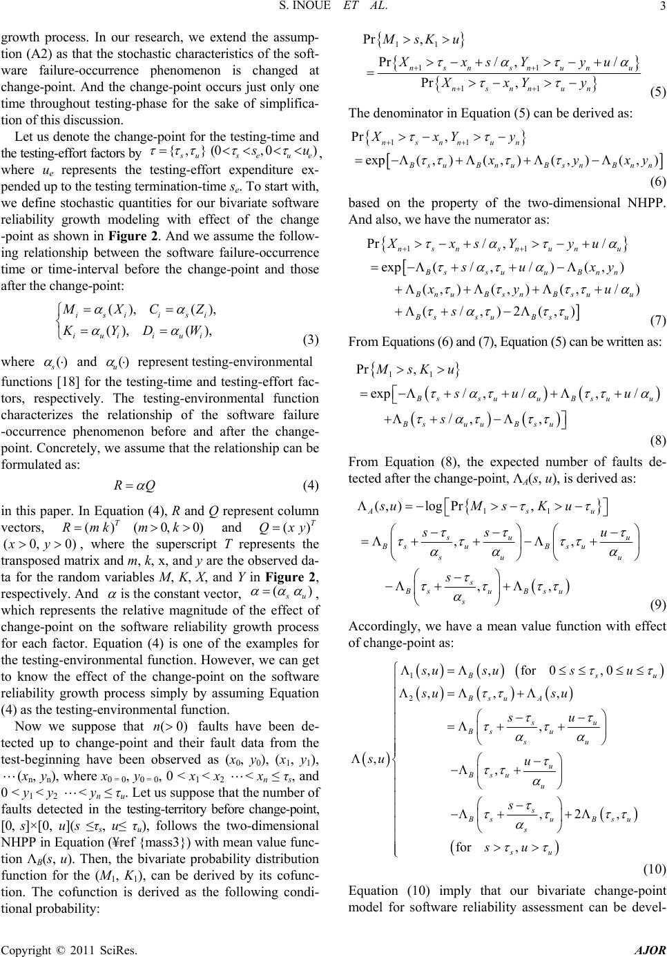 S. INOUE ET AL. 3 growth process. In our research, we extend the assump- tion (A2) as that the stochastic characteristics of the soft- ware failure-occurrence phenomenon is changed at change-point. And the change-point occurs just only one time throughout testing-phase for the sake of simplifica- tion of this discussion. Let us denote the change-point for the testing-time and the testing-effort factors by {, } u (0, 0) eue u , where ue represents the testing-effort expenditure ex- pended up to the testing termination-time se. To start with, we define stochastic quantities for our bivariate software reliability growth modeling with effect of the change -point as shown in Figure 2. And we assume the follow- ing relationship between the software failure-occurrence time or time-interval before the change-point and those after the change-point: (), (), (),( ), isi isi iui iui MXCZ KYDW (3) where () s and () u represent testing-environmental functions [18] for the testing-time and testing-effort fac- tors, respectively. The testing-environmental function characterizes the relationship of the software failure -occurrence phenomenon before and after the change- point. Concretely, we assume that the relationship can be formulated as: RQ (4) in this paper. In Equation (4), R and Q represent column vectors, and , where the superscript T represents the transposed matrix and m, k, x, and y are the observed da- ta for the random variables M, K, X, and Y in Figure 2, respectively. And () T Rmk 0) (0,0mk)() T Qxy (0,xy is the constant vector, () u , which represents the relative magnitude of the effect of change-point on the software reliability growth process for each factor. Equation (4) is one of the examples for the testing-environmental function. However, we can get to know the effect of the change-point on the software reliability growth process simply by assuming Equation (4) as the testing-environmental function. Now we suppose that faults have been de- tected up to change-point and their fault data from the test-beginning have been observed as (x0, y0), (x1, y1), (xn, yn), where x0 = 0, y0 = 0, 0 < x1 < x2 < xn ≤ τs, and 0 < y1 < y2 < yn ≤ τu. Let us suppose that the number of faults detected in the testing-territory before change-point, [0, s]×[0, u](s ≤τs, u≤ τu), follows the two-dimensional NHPP in Equation (¥ref {mass3}) with mean value func- tion ΛB(s, u). Then, the bivariate probability distribution function for the (M1, K1), can be derived by its cofunc- tion. The cofunction is derived as the following condi- tional probability: (0)n 11 11 11 Pr , Pr/ ,/ Pr , nsnsnunu nsnnun MsKu XxsYyu XxYy (5) The denominator in Equation (5) can be derived as: 11 Pr , exp(,)(,)(, )(,) nsnnun BsuBnuBsnBnn XxYy yxy (6) based on the property of the two-dimensional NHPP. And also, we have the numerator as: 11 Pr/ ,/ exp(/,/)( ,) (,)(, )(,/) (/ ,)2(,) nsnsnunu BssuuB nn nuBs nBsuu Bssu Bsu XxsYyu su xy xy u s (7) From Equations (6) and (7), Equation (5) can be written as: 11 Pr , exp/ ,/,/ /, , ssuuBsu Bsuu Bsu MsKu su u s u (8) From Equation (8), the expected number of faults de- tected after the change-point, ΛA(s, u), is derived as: 11 (,)log Pr, ,, ,, As su Bs uBsu su s Bsu Bsu s suMsK u ss u s u u u (9) Accordingly, we have a mean value function with effect of change-point as: 1 2 ,, for0,0 ,,, , ,, ,2 , for , su BsuA su Bs u su u Bsu u s BsuBsu s su su susu su su su su u s su (10) Equation (10) imply that our bivariate change-point model for software reliability assessment can be devel- Copyright © 2011 SciRes. AJOR  S. INOUE ET AL. 4 oped by assuming the two-dimensional mean value func- tion before change-point, ΛB(s, u). 4. Software Reliability A ss e s sm e n t M e a su r e Software reliability assessment measures are derived by stochastic properties of the SRGM, and play an important role in quantitative software reliability as- sessment based on the SRGM. An operational software reliability [5] is defined as the probability that a soft- ware failure does not occur in the time-interval (se, se + η](se ≥ 0, η ≥ 0) given that the testing has been going up to testing-time se and the testing-effort has been expended up to ue by testing-time se. From the basic notion of this measure and the stochastic properties in Equation (1), we can generally formulate the opera- tional software reliability as: 0 |, Pr,| , Pr , (, )1, 1,Pr ee ee ee k ee k k eee e k n ee n Rsu NsukNsu k Nsu k FsuF su n su Nn k (11) Assuming that N0 follows a Poisson distribution with parameter ω, we can derive the operational software reliability function as: |, exp,, eee eee Rsususu ) (12) by using Equation (11). 5. Parameter Estimation Parameters of our bivariate model with change-point for software reliability assessment can be estimated by the method of maximum-likelihood. Suppose that we have observed K data pairs (sk, u k, y k)(0 with respect to the number of fault yk, which have been detected in the testing-territory [0, τs]×[0, τu]+(τs, sk]×(τu, uk]. The logarithmic likelihood function, ,1,2,kK ln ,L | {(,),0,Nsu su , for the two-dimensional stochastic process given the change-point τ can be derived as: 0} 1 1 11 1 1 ln,ln,; , ,;, ,;, ln ! K kk kk k kk KK K kk k Lyysu su su yy || || (13) where θ represents the set of the parameter in Λ(s, u). Then, we obtain the following equation: ln ,ln ,0 LL || (14) The maximum-likelihood estimates are obtained by solving Equation (14) numerically. 6. Opt imal Software Release Problem If debugging cost before change-point and its after change-point a different each other, a trade-off problem between the effect of the change-point on the software reliability growth process and the related cost arises in a conventional optimal software release problem [19]. This paper discusses an optimal problem for estimating opti- mal shipping time and change-point of a software system based on our model proposed in this paper. Now, we define cost parameter for formulating the expected total software cost with change-point as fol- lows: c1: debugging cost for one fault before the change-point in the testing-phase (c1 > 0), c2: debugging cost for one fault after the change-point in the testing-phase (c2 > 0), c3: debugging cost for one fault in the operational phase (c1 < c3, c2 < c3) c4: testing cost per arbitrary testing-time and test- ing-effort (c4 > 0). Letting S, U, βs, and βu be the termination time of testing, the total testing-effort expended up to the termination time of the testing, the time duration from τs to S, and the testing-effort expended from τu to U, we have the ex- pected total software cost, C(S, U, βs, βu), as: 11 22 1 32 4 ,, ,, ,, , susu su CSUc SU cSU SU cSUcSU (15) Generally, S*, U*, βs *, and βu *, which are the cost-optimal release time, the optimal testing-effort expenditures, the optimal time duration from τs to S*, and the optimal test- ing-effort expended from τu to U*, are derived by mini- mizing the expected total software cost, C(S, U, βs, βu). Therefore, S*, U*, βs *, and βu *, are obtained by solving the following equations simultaneously: ,, ,,, , ,, ,,,,0 su su su su su CSU CSU SU CSU CSU (16) We should note that Equation (16) is a necessary condi- tion for the optimal solutions. Equations (15) and (16) can be simplified to an optimal testing-effort expending problem for estimating optimal testing-effort expendi- Copyright © 2011 SciRes. AJOR  S. INOUE ET AL. 5 Figure 3. Estimated two-dimensional mean value function with effect of change-point, 6 12.89 su τ=,τ= Figure 4. Estimated operational software reliability, ˆ(19, 47.65)Rη| tures in the restricted testing-time. The expected total software cost for the optimal testing-effort expending problem is derived as: 52324 ,,, ,, su CSU cSUc SUcS U (17) where S, , and u represent the given testing-time duration, βs, and βu, respectively. And c5 is the debugging cost for one fault in the testing-phase, in which we as- sume that there is no difference between the debugging cost for one fault before and after the change -point. From the basic notion in Equation (16), the optimal test- ing-effort expenditures U* needs to satisfy the following equation: 3 21 2 321 (, ,,)(, )0 su CSU c cc ShSU Uccc (18) where 22 ,,hSUSUU . 7. Numerical Examples We show numerical examples of our bivariate model and its application to an optimal software release problem. In this paper, we use actual data consisted of 19 data pairs: (sk, uk, yk)(k = 0, 1, 2,…,19; t19 = 19(weeks), s19 = 47.65(CPU hours, y19 = 328) [20]. And we assume that the software failure-occurrence time distribution before change-point follows the following bivariate probability distribution function [21]: ,1e1e1e 0,0, 11 asbsas bu Fsu z ab z (19) And we set αs =αu = α for simplification and we also set , 6,12.89 su τ by following the actual behav- ior of the software failure-occurrence phenomenon. Then, we estimate the parameters as ˆ, , , a ˆb ˆ ˆ, and ˆ, which are the estimates of , , , ab , and α by the method of maximum likelihood discussed in Section 5. Figure 3 shows the two-dimensional behavior of the estimated mean value function with effect of the change-point, where τs = 6, τu = 12.89. In Figure 3, the dotted line represents the actual behavior of the cumula- tive number of detected faults and the curved surface the estimated behavior. We see that the expected number of faults is estimated to be zero outside the software fail- ure-occurrence territory, which has been explained in Figure 2. This is one of the feature for our two -dimensional SRGM with the effect of the change-point. Further, Figure 4 shows the estimated operational soft- ware reliability, . From Figure 4, we can estimate the operational software reliability at 0.3 weeks after the termination time of the testing, , to be about 0.036. )65.47,19|( ˆ R )65.47,19|3.0( ˆ R Then, we show numerical examples for an optimal re- lease problem for deriving optimal testing-effort expen- diture based on our bivariate change-point model. This problem is one of the simplified problem for our optimal software release problem. In this problem, 2(,)hSU in Equation (19) can be derived as: 2 2 11 , , exp exp u SU hSUU bbDUBbD UA (20) where 22 2exp[]exp[2](1)exp[] zaDz aDza p[ 2] ex za 22 2exp[]2exp[2]Bz aDzaD, xp[]2exp[ 2] 2 e s zaz a , 1() , u u u U DU respectively. We can easily see that U* can be obtained by solving the following equations: 4 2 35 , cShSU cc (21) Copyright © 2011 SciRes. AJOR  S. INOUE ET AL. 6 Table 1. Sensitivity analysis of the optimal testing-effort expenditures. 5 c 3 c 4 c * U * (,,,) u CSU 1 5 5 3.2501 5117.1 1 5 3 10.856 4021.2 1 5 1 28.840 2925.3 1 10 1 43.318 5029.7 1 20 1 57.253 9238.6 1 40 1 70.975 17656 1 80 1 84.606 34492 Figure 5. Time-dependent behavior of the estimated ex- pected total software cost and ˆ2 hS,U . (τs = 6, τu = 12.89, c5 = 1, c3 = 5, and c4 = 1). Table 1 shows the results of the sensitivity analysis of the optimal testing-effort expenditures. From Table 1, we can say that the optimal testing-effort expenditures are getting increased as the debugging cost for one faults in the operational phase is increased. On the other hand, the optimal testing-effort expenditures are also getting increased as the testing cost per arbitrary testing-time and testing-effort is decreased. Further, Figure 5 shows the computed results for the time-dependent behavior of the expected total software cost and 2 ˆ(,)hSU, where c5 = 1, c3 = 5, and c4 = 1. From Figure 5, we can estimate the optimal testing-effort expenditures, U*, and the ex- pected total software cost, ),,,(* us USC to be about 28.84 (CPU hours) and 2925.33, respectively. 8. Concluding Remarks This paper discussed a bivariate software reliability growth modeling with the effect of the change-point and an optimal software release problem based on our model. Further, we showed numerical examples of software re- liability analysis and an optimal testing-effort expending problem based on our model by using actual data. Our bivariate SRGM with the effect of change-point is ex- pected to contribute high accuracy assessment of soft- ware reliability in a testing-phase. In the further studies, we have to investigate the effectiveness and validity of our model by using a lot of data sets collected from ac- tual software development projects, and have to give a discussion on sufficient conditions for the optimal soft- ware release problem. 9. Acknowledgement This work was supported in part by the Grant-in-Aid for Scientific Research (C), Grant No. 22510150, from the Ministry of Education, Sports, Science, and Technology of Japan. 10. References [1] J.D. Musa, “A theory of software reliability and its ap- plication,” IEEE Transactions on Software Engineering, Vol. SE-1, No. 3, 1975, pp. 312-327. [1] S. Yamada and S. Osaki, “Software reliability growth modeling: Models and applications,” IEEE Transactions on Software Engineering, Vol. SE-11, No. 12, 1985, pp. 1431-1437. doi:10.1109/TSE.1985.232179 [2] J.D. Musa, D. Iannio, and K. Okumoto, “Software Reli- ability: Measurement, Prediction, Application,” McGraw -Hill, 1987. [3] H. Pham, “Software Reliability,” Springer-Verlag, 2000. [4] T. Ishii and T. Dohi, “Two-dimensional software reliabil- ity models and their application,” Proceedings of the 12th Pacific Rim International Symposium on Dependable Computing, 2006, pp. 3-10. [5] S. Inoue and S. Yamada, “A bivariate Weibull-type soft- ware reliability growth model and its goodness-of-fit evaluation,” (in Japanese) J. Information Processing So- ciety of Japan, Vol. 49, no. 8, August 2008, pp. 2851 Copyright © 2011 SciRes. AJOR  S. INOUE ET AL. Copyright © 2011 SciRes. AJOR 7 -2861. [6] S. Inoue and S. Yamada, “A framework for two-dimensional software reliability modeling with pro- gram size,” Proceedings of the 14th ISSAT International Conference on Reliability and Quality in Design, 2008, pp. 198-202. [7] M. Zhao, “Change-point problems in software and hard- ware reliability,” Communications in Statistics -- Theory and Methods, Vol. 22, No. 3, 1993, pp. 757-768. doi:10.1080/03610929308831053 [8] C.Y. Huang, “Performance analysis of software reliability growth models with testing-effort and change-point,” Journal of Systems and Software, Vol. 76, No. 2, 2005, pp. 181-194. doi:10.1016/j.jss.2004.04.024 [9] C.Y. Huang, “Cost-reliability-optimal release policy for software reliability models incorporating improvements in testing efficiency,” Journal of Systems and Software, Vol. 77, No. 2, 2005, pp. 139-155. doi:10.1016/j.jss.2004.10.014 [10] F.Z. Zou, “A change-point perspective on the software failure process,” Software Testing, Verification and Reli- ability, vol. 13, no. 2, 2003, pp. 85-93. doi:10.1002/stvr.268 [11] J. Zhao, H.W. Liu, G. Cui, and X.Z. Yang, “Software re- liability growth model with change-point and environ- mental function,” Journal of Systems and Software, Vol. 79, No. 11, 2006, pp. 1578-1587. doi:10.1016/j.jss.2006.02.030 [12] S. Inoue and S. Yamada, “Software reliability measure- ment with change-point,” Proceedings of the International Conference on Quality and Reliability, 2007, pp. 170 -175. [13] S. Inoue and S. Yamada, “Optimal software release pol- icy with change-point,” Proceedings of the IEEE Interna- tional Conference on Industrial Engineering and Engi- neering Management, 2008, pp. 531-535. doi:10.1109/IEEM.2008.4737925 [14] N. Langberg and N.D. Singpurwalla, “A unification of some software reliability models,” SIAM Journal on Sci- entific Computing, Vol. 6, No. 3, 1985, pp. 781-790. doi:10.1137/0906053 [15] D.S. Miller, “Exponential order statistic models of soft- ware reliability growth,” IEEE Transactions on Software Engineering, Vol. SE-12, No. 1, 1986, pp. 12-24. [16] D.N.P. Murthy, J. Baik, R.J. Wilson, and M.R. Bulmer, “Two-dimensional failure modeling,” In: H. Pham, Ed., Springer Handbook of Engineering Statistics, Springer -Verlag, Berlin, 2006, pp. 97-111. doi:10.1007/978-1-84628-288-1_5 [17] H. Okamura, T. Dohi, and S. Osaki, “A reliability as- sessment method for software products in operational phase? Proposal of an accelerated life testing model,” (in Japanese), Transactions of IEICE, Vol. J83-A, No. 3, 2000, pp. 294-301. [18] S. Yamada and S. Osaki, “Cost-reliability optimal release policies for software systems,” IEEE Transactions on Re- liability, Vol. R-34, No. 5, 1985, pp. 422-424. doi:10.1109/TR.1985.5222222 [19] M. Ohba, “Software reliability analysis models,” IBM Journal of Research and Development, Vol. 28, No. 4, 1984, pp. 428-443. doi:10.1147/rd.284.0428 [20] E.J. Gumbel, “Bivariate exponential distributions,” Journal of the American Statistical Association, No. 55, 1960, pp. 698-707. doi:10.2307/2281591
|