Applied Mathematics, 2011, 2, 363-368
doi:10.4236/am.2011.23043 Published Online March 2011 (http://www.SciRP.org/journal/am)
Iterated Logarithm Laws on GLM Randomly Censored
with Random Regressors and Incomplete Information#
Qiang Zhu1, Zhihong Xiao1*, Guanglian Qin1, Fang Ying2
1Statistics Research Institute, Huazhong Agricultural University, Wuhan, China
2School of Science, Hubei University of Technology, Wuhan, China
Received December 8, 2010; revised January 26, 2011; accepted Janu ary 29, 2011
Abstract
In this paper, we define the generalized linear models (GLM) based on the observed data with incomplete
information and random censorship under the case that the regressors are stochastic. Under the given condi-
tions, we obtain a law of iterated logarithm and a Chung type law of iterated logarithm for the maximum li-
kelihood estimator (MLE) ˆn

in the present model.
Keywords: Generalized Linear Model, Incomplete Information, Stochastic Regressor, Iterated Logarithm
Laws
1. Introduction
The generalized linear model(GLM) was put forward by
Nelder and Wedderburn [1] in 1970s and has been stu-
died widely since then. The maximum likelihood esti-
mator (MLE) ˆn

of the parameter vector

in GLM
was given and its strong consistency and asymptotic
normality were discussed by Fahrmeir and Kaufmann [2]
in 1985.The randomly censored model with the incom-
plete information was presented by Elperin and Gertsba-
kin [3] in 1988.The analysis of the randomly censored
data with incomplete information has become a new
branch of the Mathematical Statistics. Xiao and Liu [4]
in 2008 discussed the strong consistency and the asymp-
totic normality of MLE ˆn

of GLM based on the data
with random censorship and incomplete information.
Xiao and Liu [5] discussed laws of iterated logarithm for
quasi-maximum likelihood estimator of GLM in 2008,
meanwhile, Xiao and Liu [6] in 2009 discussed laws of
iterated logarithm for maximum likelihood estimator of
generalized linear model randomly censored with in-
complete information under the regressors given. How-
ever, Lai and Wei [8], Zeger and Karim [9] have studied
the linear regression model under the case that the re-
gressors are stochastic. In the practical application, espe-
cially in the biomedical social sciences, the regressors in
GLM are often stochastic, Fahrmeir [10] investigated
GLM with the regressors 1,,n
X
Xwhich are indepen-
dent and identically distributed and gave MLE of matrix
parameter without proof under the given conditions.
Ding and Chen [11] in 2006 gave asymptotic properties
of MLE in GLM with stochastic regressors. So, in the
present paper, we will investigate the law of iterated lo-
garithm and the Chung type law of iterated logarithm for
maximum likelihood estimator of generalized linear mo-
del randomly censored with incomplete information un-
der the case that regressive variables,1
i
X
iare inde-
pendent but not n ecessarily identically distributed.
From a statistical perspective, the importance of those
laws stem from the fact that the first one gives in an asy-
mptotic sense the smallest 100% confidence interval for
the parameter, while the second one gives an almost sure
lower bound on the accuracy that the estimator can achi-
eve.
2. Model with the Random Regressor
Suppose that the respondence variables ,1,2,,
i
Yi n


are one dimension random variables, and regressor vari-
able ,1,2,,
i
X
in

 are q-dimension r andom variables
which have the distribution functions ,1,2,,
i
Kires-
pectively. Here, i
x
is the observation value ofi
X
, i
X

i

. Write 1ii



. Suppose that the observations


,,1,2,,
ii
YX iare mutually independent and satisfy.
*Correspondin g Au tho r.
#Foundation items: supported by Huazhong Agricultural University
Doctoral Fund (52204-02067) and Interdisciplinary Fund (2008 xkjc008
and Torch Plan F und (2009XH003).

Q. ZHU ET AL. 364
1) The regression equation:



|,1
T
ii ii
EY Xxmxi    (2.1)
where the unknown parameter .
q
B  
2) The conditional distribution of i Y under ii
X
x

is
the exponent distribution, i.e.






exp, 1
iiiii
P
YdyX xCyybdyi   
(2.2)
where

is a

-finite measure, parameter i


,

1, 2,,in,
 

:0 expCyy dy   

is the natural parameter space and 0
is the interior of
. Since this conditional density integrates to 1, we see
that
 
exp
ii
bC ydy  , from which the
standard expressions for the conditional mean




|
ii ii
EY Xxb


, and the variance,


|
ii i
Var YXx

i
b

 ， where

,b


b
  denote the first and second
derivatives of

b, respectively.
Suppose that the censor random variables ,
i
U i

1, 2,, n are mutually independent but not necessarily
identically distributed, with the distribution function

i
Gu and
 


ii
dG ugudu  . Denote


i
K
dx

 
,
i
x
dx  1, 2,,in. Suppose that i U is indepen-
dent of

,
ii
YX
For 1, 2,,in, let

ii
iYU
I


,
0,if ,but the real va isn't observed ,lue of
1,else,
i
iii
UYY





,if 1,1
,otherwise
ii i
ii
Y
ZU






Obviously,
 
,,,,1,2,
iii i
ZXi   is a mutually
independent and observable sample. The conditional
density and distribution function of i Y underii
X
x

are respectively denoted as





;exp
TTT
iii
fyxCyx ybx

 


 


;exp
|
z
TTT
iii
iii
F
zxC yxybxdy
PYzXx



 

Let
 
1,
ii
Gz Gz




;1;
TT
ii
Fzx Fzx

  , 1, 2,,in.
Suppose


,1| ,,
if ,,
ii i i
i
P
YyUuXxp
yu x
   
 (2.3)


0|,,1 ,
if ,,
ii ii
i
YyU uXx
yu x
P
p  
 (2.4)
where 01p

. This assumption came from T. Elperin
and I. Gertsbak, [3]. In the reliab ility study, the instant of
an item's failure is observed if it occurs before a ran-
domly chosen inspection time and the failure is signaled.
Otherwise, the experiment is terminated at the instant of
inspection during which the true state of the item is dis-
covered. T. Elperin and I. Gertsbak, assumed that the fai-
lure time of every item was signaled randomly with p ro-
bability p before the rando mly chosen inspectio n time.
Then, we have




,
,,,
iii
ii i
PY yU uXx
P
YyXxPUu yux

 
Without loss of generality, assuming that i
X
is dis-
crete, we have




iiiii i
PYy,UuXxPYyXxPUu

 
(2.5)
We first give the following propositions.
Proposition 2.1. Under the regular assumptions above,
we have


 
,1,1|
,
iii i
z
ii
PZ zXx
pGyfy dy




 
 (2.6)





,1,0|
1;,
iii i
zT
iii
PZ zXx
pFyxdGy




 
  (2.7)




,0|
;.
ii i
zT
iii
PZ zXx
F
yxdG y





 (2.8)
Proof. We only show (2.6) for the discrete case, the
continuous case can be shown in the way similar to that
of the discrete case.




,1,1 ,,
1
1,, ,
ii iiiiiiii
iiii
z
ii i iiiiii
y
zz
ii ii
PZzX x EIIEIYUX xX x
YzYU
PYyUuXxP YdyUduXx
pGydFypGyfydy
 




 



 



 







(2.9)

Q. ZHU ET AL. 365
where (2.9) follows from (2.3) and (2.5). Similarly, we
can demonstrate (2.7) and (2.8).
Suppose that i zis the observation of i
Z
,i

is the
observation of i

, i

is the observation of i

, (2.6),
(2.7) and (2.8) imply that for all 1i, the conditional
distribution of

,,
iii
Z

 under ii
X
xis the follow-
ing






(1 )
1
( )(;)][(1)(;)()
;
ii
ii
i
TT
ii iiii ii
T
iii ii
pGzfzxpFzx gz
Fzxgzdz













(2.10)
Let


1,, , n
n
Z
ZZ


1,, , n
n
zzz


1,, , n
n
 


1,, , n n
 


1,, , n n

 


1,, , n
n

 



12
,,,XXX



1,,
,
n
n
X
XX


1,, , n
n
x
xx


12
,, .xxx

We easily get the following proposition.
Proposition 2.2. For all 1n, we have
 


 


,,
,,
,,
1
nnn nnn
nnn nnnnn
iii iiiii
PZ zX x
PZ zXx
nPZ zXx
i
 
 



 


(2.11)
and


 

 
,,
,,
(, ,),1,
iii iii
iii iii
nn
iii iii ii
PZ zXx
PZ zXx
PZ zXxi


 

 
 

 
(2.12)
where () ()nn
Z
z

means ii
Z
z for 1in .
Remark 2.1. Proposition 2.2 implies that under


|,,1
i
PX xUi


 are mutually independent and so
are ,1
i
Yi, and


,,, 1.
iii
Zi  
(2.10) and (2.11) imply that the conditional distribu-
tion of






111
,, ,,,,
nnn
ZZ    under
  nn
X
x

is







 
1
1
1
;,1;1;
iii i
nTT T
i iiiiii iiiii
ii
Fxgd n
i
pGzfzxp Fzxgzzzz
  




 



 


 
 (2.13)
The conditional probability measure corresponding to
(2.13) is written as


|.PXx
 
Meanwhile, let

x
E

 and

x
Var

 denote the conditional expecta-
tion and conditional variance under the conditional pro-
bability measure

|,PXx
 
respectively. Set 0

do-
note the real value of

. For notational simplicity, let




xx
EE


 and
 
xx
Var Var


. (2.13) im-
plies that the joint distribution of is






111 1
,,,,, ,,,
nnnn
ZXZ X   







 
11
1;1; ;
iii i
i
nTT T
i iiiiii iiii iiiii
ipGzfzxpFzxgzF zxgzdzxdx
 
 


 


 

 
 (2.14)
The probability measure (unconditional) correspond-
ing to (2.14) is denoted as

P

. Meanwhile, let

E

 and

Var

 denote the expectation and vari-
ance under the probability measure

P

, respectively.
For notational simplicity, let
 
,PPEE

  and



Var Var


It is that the parameters in (2.14) are studied by us.
3. Main Results
Furthermore, from (2.14) we get the likelihood function
of





111 1
,,,,, ,,,
nnnn
ZXZ X   
as follows

1111
,,,, ,,,,,
nnnn
LZX ZX   





 

  
1
;
1
1
1;
;,1
i
ii
T
ii ii
Tii
ii ii
T
iiiii i
npGZf ZX
i
pFZ XgZ
FZXgZXn













 





 (3.1)
Taking the logarithm to (3.1) and dropping the terms
which are free of

yield the logarithm likelihood fun-
ction:








*
1
1111
log ;1
log;1 log;
;,,, ,,,,,,
nT
niiiiii
i
TT
iii ii
nnnnn
lfZX
FZX FZX
lZ XZX
 


 




 



(3.2)
where


1111
;,,,,,,,,
nnnnn
lZ xZx    is the loga-
rithm likelihood function defined in Xiao and Liu [8].

Q. ZHU ET AL. 366
We have the score function
 











**
1
1111
1;
;
1;;,,,,,,,,,
;
i
i
Z
nii
TT
nn iiiiiii
iT
iii
iT
ii nnnnn
TZ
ii
Tl XZbXyfyXdy
FZX
yfyXdyTZXZX
FZX

 

 





 








(3.3)
where

1111
;,,, ,,,,,
nnnnn
TZ XZX   is defined as in Xiao an d Liu [8]. And

 
















2* 2
*
12
2
2
2
2
111
1
=1 ;
;
11
;1 ;
;;
1;
;
;,,
i
i
i
i
Z
n
nTT T
iiiiii i
nTiT
iii
ZTT
ii iii
TT Z
iiii ii
T
ii
TZ
iii
n
l
HXXbX yfyXdy
FZX
yf yXdyyf yXdy
FZXF ZX
yf yXdy
FZX
HZ


 
 










 

 



















1
,,, , ,,
nnnn
xZ x  
where

1111
;,,,,,,,,
nnnnn
H
ZxZ x    is defined
as in Xiao and Liu [8]. Write


 

** **
1
;,, T
x
nnn nn
xxET T

 








*1
;,, ,
xnn n
EHx x



 
where

1
;,,
nn
x
x   is defined as in Xiao and Liu
[8].
The solution of the log arithm lik elihood equation

*0
n
T 

(3.4)
is written as

1111
,,, ,,,,,.
nn nnnn
Z
XZ X   
  (3.5)
(3.3) and (3.4) imply that

111 1
ˆ,,,,,,,,,
nn nnnn
ZXZ X   
 (3.6)
where

1111
ˆ,,, ,,,,,
nnnnn
Z
XZ X    is defined as
in Xiao and Liu [8]. The norm of matrix

ij
p
q
Aa

 is
defined as 2.
11
pq
A
aij
ij

 We write , as the
usual inner product and
s
e as the sth canonical basis
in q . Let

1
1,,;
z
zFzyfydy 


 
 
12
2,, ;
z
zFzyfydy  


 
 
1
3,,;
z
zFz yfy dy 


 
 
12
4,, ;
z
zFz yfy dy  


 
and

 
|.
T
nnn nn
ET TXx




 


We state the following assump tions:
(1C) For all 1i, for all B

，0,
T
i
X 

a.s.,
where i X

. Here

is compact.
(2C)





1
00
;lim;
nn
n
QXnX 


 is a q-order
positive define matrix.
(3C) For all12 ,B



,





22
1112112
;; ,,
TT
zxzxL zx

   (3.7)





21222 12
;; ,,
TT
zxzxLzx

   (3.8)





22
31323 12
;; ,,
TT
zxzxL zx

   (3.9)





41424 12
;; ,,
TT
zxzxLzx

   (3.10)
where


1
sup;,. .1,2,3,4,1.
bT
iji j
EL ZxXLasjb



 

(4C)

2
,1, 0,
XT
i
BiEt X




 

a.s.
It is also easy to see that the conditions in the present
paper imply the conditions (C1), (C2), (C3) and (C4)
given in Xiao and Liu[8]. So, there almost sure exists the
maximum likelihood estimator of0

. Hence, our first
result states a law of the iterated logarithm for the max-
imum likelihood estimator of 0

.
Theorem 3.1. Under conditions (1C), (2C), (3C)
and (4C), if ˆn

is the MLE of 0

, then for 1
s
q

,
we have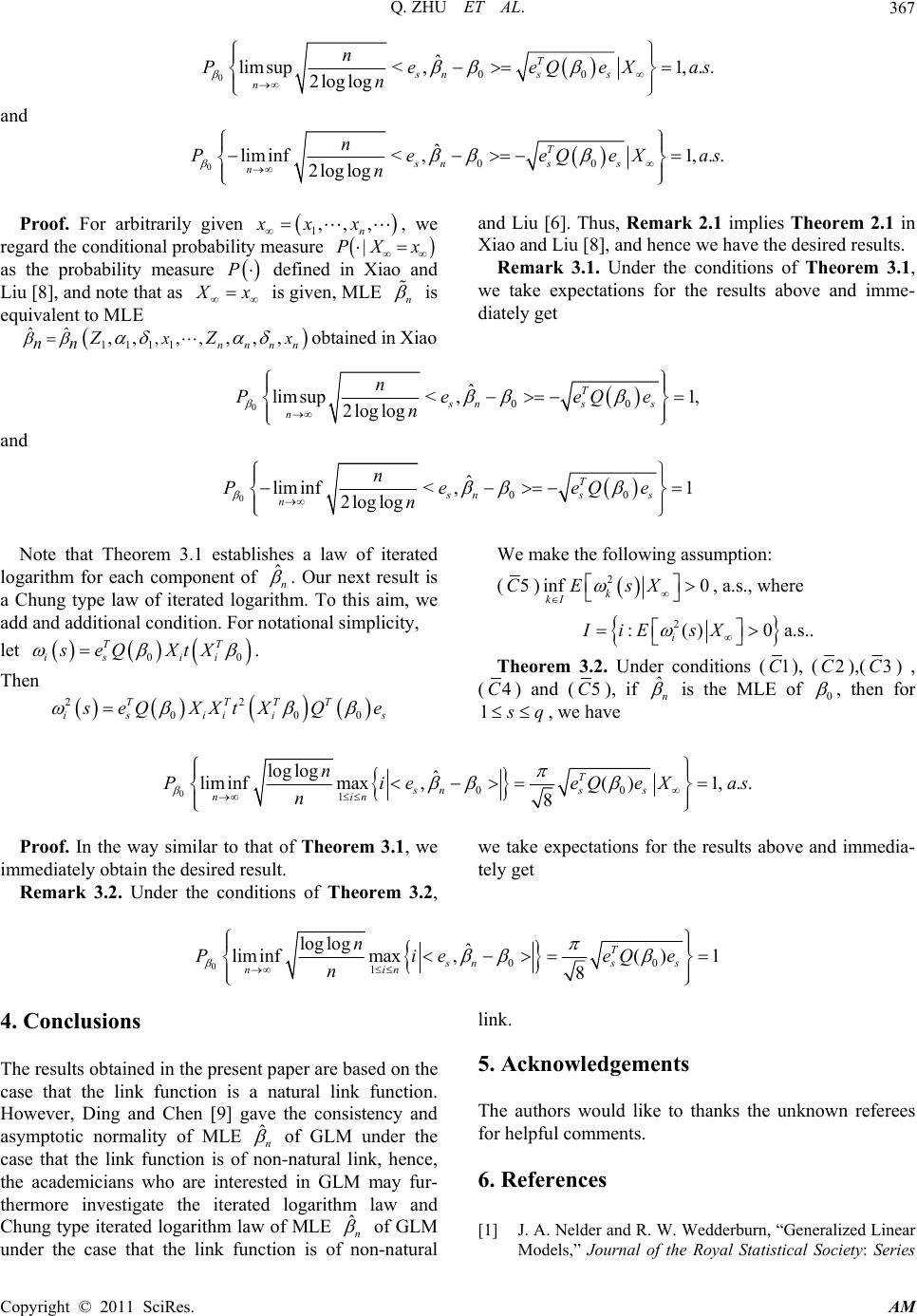

Q. ZHU ET AL. 367

000
ˆ
limsup,1,. .
2log log
T
snss
n
n
P<eeQeXas
n

 




 



and

000
ˆ
liminf,1,..
2loglog
T
sns s
n
n
P<eeQeXas
n

 








Proof. For arbitrarily given

1,,, n
xxx
, we
regard the conditional probability measure


|PX x



as the probability measure


P defined in Xiao and
Liu [8], and note that as
X
x


is given, MLE n

 is
equivalent to MLE

1111
ˆˆ ,,,
,, ,,,
nnnn
x
x
nn
ZZ    obtained in Xi ao
and Liu [6]. Thus, Remark 2.1 implies Theorem 2.1 in
Xiao and Liu [8], and hence we have the desired results.
Remark 3.1. Under the conditions of Theorem 3.1,
we take expectations for the results above and imme-
diately get

000
ˆ
limsup ,1,
2log log
T
sns s
n
n
P<eeQe
n

 




 



and

000
ˆ
liminf ,1
2log log
T
sns s
n
n
P<eeQe
n

 







Note that Theorem 3.1 establishes a law of iterated
logarithm for each component of ˆn

. Our next result is
a Chung type law of iterated logarithm. To this aim, we
add and additiona l condition. For notational simplicity,
let
 

00
TT
is ii
seQXtX

 .
Then




22
000
TTTT
is iiis
s
eQXXt XQe   
We make the following assumption:
(5C)


2
inf 0
k
kIEsX





, a.s., where


2
:() 0
i
IiE sX 





a.s..
Theorem 3.2. Under conditions (1C), (2C),( 3C) ,
(4C) and (5C), if ˆn

is the MLE of 0

, then for
1
s
q

, we have

000
1
loglog
liminfmax, ˆ() 1,..
8
T
sns s
nin
n
PieeQeXas
n


 

 


 



Proof. In the way similar to that of Theorem 3.1, we
immediately obtain the desired result.
Remark 3.2. Under the conditions of Theorem 3.2,
we take expectations for the results above and immedia-
tely get

000
1
loglog
liminfmax,( )1
8
ˆT
sss
nin n
n
PieeQe
n



 



 



4. Conclusions
The results obtained in the present paper are based on the
case that the link function is a natural link function.
However, Ding and Chen [9] gave the consistency and
asymptotic normality of MLE ˆn

of GLM under the
case that the link function is of non-natural link, hence,
the academicians who are interested in GLM may fur-
thermore investigate the iterated logarithm law and
Chung type iterated logarithm law of MLE ˆn

of GLM
under the case that the link function is of non-natural
link.
5. Acknowledgements
The authors would like to thanks the unknown referees
for helpful co mments.
6. References
[1] J. A. Nelder and R. W. Wedderburn, “Generalized Linear
Models,” Journal of the Royal Statistical Society: Series

Q. ZHU ET AL. 368
A, 135, Part 3, 1972, pp. 370-384. doi:10.2307/2344614
[2] L. Fahrmeir and H. Kaufmann, “Consistency and Asym-
totic Normality of the Maximum Likelihood Estimator in
Generalized Linear Models,” Annals of Statistics, Vol. 13,
No. 1, 1985, pp. 342-368. doi:10.1214/aos/1176346597
[3] T. Elperin and I. Gertsbak, “Estimation in a Random
Censoring Model with Incomplete Information: Expo-
nential Lifetime Distribution,” IEEE Transactions on Re-
liability, Vol. 37, No. 2, 1988, pp. 223-229.
doi:10.1109/24.3745
[4] T. L. Lai and C. Z. Wei, “Least Squares Estimates in
Stochastic Regression Models with Applications to Iden-
tification and Control of Dynamic Systems,” Annals of
Statistics, Vol. 10, No. 1, 1982, pp. 154-186.
doi:10.1214/aos/1176345697
[5] S. L. Zeger and M. R. Karim “Generalized Linear Models
with Random Effects; A Gibbs’ Sampling Approach,”
Journal of the American Statistical Association, Vol. 86,
No. 413, 1991, pp. 79-86. doi:10.2307/2289717
[6] Z. H. Xiao and L. Q. Liu, “MLE of Generalized Linear
Model Randomly Censored with Incomplete Informa-
tion,” Acta Mathematica Scientia, Vol. 3(A), 2008, pp.
553-564.
[7] Z. H. Xiao and L. Q. Liu. “Laws of Iterated Logarithm
for Quasi-Maximum Likelihood Estimator in Generalized
Linear Model,” Journal of statistical planning and infe-
rence, Vol. 138, No. 3, 2008, pp. 611-617.
doi:10.1016/j.jspi.2006.12.006
[8] Z. H. Xiao and L. Q. Liu, “Laws of Iterated Logarithm
for MLE of Generalized Linear Model Randomly Cen-
sored with Incomplete Information,” Statistics and
Probability Letters, Vol. 79, No. 6, 2009, pp. 789-796.
doi:10.1016/j.spl.2008.11.016
[9] J. L. Ding and X. R. Chen, “Asymptotic Properties of the
Maximum Likelihood Estimate in Generalized Linear
Models with Stochastic Regressors,” Acta Mathematica
Sinica, Vol. 22, No. 6, 2006, pp. 1679-1686.
doi:10.1007/s10114-005-0693-3