Applied Mathematics, 2011, 2, 355-362
doi:10.4236/am.2011.23042 Published Online March 2011 (http://www.SciRP.org/journal/am)
Existence of Periodic Solution for a Non-Autonomous
Stage-Structured Predator-Prey System with Impulsive
Effects
Lifeng Wu, Zuoliang Xiong, Yiping Deng
Department of Mathematics, Nanchang University, Nanchang, China
Received November 20, 2010; revised January 25, 2011; accepted Ja nu ary 28, 2011
Abstract
In this paper, we studied a non-autonomous predator-prey system where the prey dispersal in a two-patch
environment. With the help of a continuation theorem based on coincidence degree theory, we establish suf-
ficient conditions for the existence of positive periodic solutions. Finally, we give numerical analysis to show
the effectiveness of our theoretical results.
Keywords: Periodic Solution, Coincidence Degree Theory, Stage-Structured, Impulsive
1. Introduction
In recent years, non-autonomous predator-prey systems
have been widely studied [1-6]. There has been a grow-
ing interest in the study of mathematical models of pop-
ulations dispersing among patches in the nature world
[3,7-9].
In the classical predator-prey models it is usually as-
sumed that each individual predator admits the same abi-
lity to feed on prey. However, it is different for some
species whose individuals have a life history that takes
them through two stages, immature and mature, where
immature predators are raised by their parents, so many
models with time delays and stage structure for both prey
and predator were investigated and rich dynamics have
been observed [4,6,10-12].
In this paper, we are considered the effects of prey dif-
fusion in two patches and maturation delay for predator
on the dynamics of an impulsive predator-prey model.
We discuss the differential equation: (See 1.1)
Where we suppose that the system is composed of two
patches connected by diffusion.

1
x
tand


2
x
t repre-
sent the densities of prey species in patch I and II at time t,

1
y
t and

2
y
trepresent the densities of the imma-
ture and mature predator at time t in patch II , respectively .

1,
x
t

2
x
tcan diffuse between patch I and II while the
predator species is confined to patch II.

repre- sents a
constant time to maturity.

 
1, 2
i
atiis the intrinsic
 


  
  

  
 
 
 
 
 

11111
12 1
22222
22
21 2
122
()
22
2
111
()
222
2
22
11
,
,,
,
,
1
t
t
t
t
k
rsds
rsds
k
xtxt atrtxt
dtxt xt
xtxtat rtxt
ktx tyt
dtxt xttt
yt ctxtyt
ctex ty t
dty tq tyt
yt ctextyt
qtyt
xt













 
 
 



 




 


 

 















1
222
1122
,
1, ,
1, ,
kk
kkkk
kkkkk
xt
xtxtt t
ytyt ytyt


























  


 


(1.1)
growth rate;




1, 2
i
i
rt i
at is the carrying capacity;




1, 2
i
dti is the dispersal rate of prey species;


ktis the captur e rate of mature predator.


ctis a co n-
version efficiency.


dtis the death rate of the imma-
ture predator.




1, 2
i
qti is the rate of intra-specific

L. F. WU ET AL. 356
competition. ik

and k

represent the annual birth pul-
se of
 
1
,1,2
i
xt ytiat

k
tkZ

. We make the
following assumptions fo r o u r m odel:
1)
















,, ,1,2,,,
iii i
atrtdtqti dtktctand

rtare continuous positive


periodic functions；
2) 12
,
kk

 and k

are constants and there exists a po-
sitive integerqsuch that
112 2
,,,
kqkkqkkqk kqk
tt

 



.
2. Preliminaries
Denote by
 
,PCJ RJRthe set of functions :

J
R, which are piecewise continuous in


0,

, and
have points of discontinuity


0, .
k
t

 Let


1,PCJR
denote the set of functions

with derivative


t 



,PCJ R. We define the Banach space of


periodic
functions




 

0, ,0PCPC R


   with
 

sup: 0,
PC tt

 and 1 PC

with 1
PC





1
max( ),
PC PC
t



, we will considered the
P
CPC


with the norm
12
(, )
PC
 12
P
CPC
 .
We define:

0
1
f
ftdt


,

[0, ]
min
L
t
f
ft
 
,


[0,]
max
M
t
f
ft
 
.
3. Existence of Positive Periodic Solutions
In this section, we study the existence of positive period-
ic solutions of system (1.1).
Before stating our result on positive

periodic solu-
tions of system (1.1), we need the following lemma:
Lemma 3.1 ([13]). Let
X
 be an open bounded set.
Let L be a Fredholm mapping of index zero and N
be Lcompact on . Assume
1) for each

0,1  ,
x
is any solution ofLxNx


such thatx;
2) for each0QNx for each
x
KerL ;
3)

deg,,0 0JQN KerL .
Then the equation Lx Nx has at least one solution
in DomL .
Theorem 3.1 If the system (1.1) satisfies
(H1)

1
ln 10
q
k
k
a 





,

1
ln 10
q
k
k
d 






,
(H2)

11 1
ln 10
q
k
k
ad 






,

4
22 2
1
ln 10
q
M Mk
k
ad ke  






,
(H3) 242 40
L
mmr MM LM
cec e


,
then the system (1.1) has at least one

periodic posi-
tive solution.
Proof. Let






123
12 1
,,,
utut ut
xt ext eyt e


4
2ut
yt e, then
 


 

 




 

 
 
 


 
 
 


121
24
12
243 3
243
244
4
1111
1
222
22
31
4
2
,
,
,
,
t
t
t
t
utut ut
ut ut
ut ut
ututut ut
rsds ut ut ut
rsds ut ut ut
ut
utatrtedte
dt
utatrtekte
dte dtt
utctedtqte
ct ee
ut ctee
qte











 
 



 


 

 






 

 







,
k
t



















 

 

 


11 1
22 2
33 44
ln 1,
ln 1,,
ln 1,,
kk k
kk kk
kk kkk
ut ut
ut uttt
ut utut ut











 


 



(3.1)
One can easily see that if system (3.1) has one


periodic solution
 

1234
,,, T utututut, then
  


 

12341212
,,,, ,,
TT
ut ut utut
e eeextxtytyt


is a positive


periodic solution of system(1.1). Thus,
in what follows our goal is to show that system (3.1) has
at least one


periodic sol ut i on.
Here, we rew rite




1122
,,
f
tutftut





3344
,
f
tutftut

.
Let
111
DomLPC PCPC



and
111
:NPCPCPC Z

 ,
with

L. F. WU ET AL. 357







1
11
2
22
33
41
4
ln 1
ln 1
,ln 1
0
q
k
k
k
k
ft
u
ft
u
Nuft
uft






 



 
 






 
 


 


  

and

11 1
22 24
33 3
44 4
:,0,
uu C
uu C
KerLR t
uu C
uu C



 











.
Where Q is defined by




01
01
011
01
0
0
1,0
0
q
k
kq
q
k
kq
k
kk
q
k
k
ftdt a
gtdt b
QZ
htdtc
jtdt d































 























.
Furthermore, :Im
P
K
LKerPDomL is given by
 
 
 
 
000
01
000
01
000
01
000
01
1
1
1
1
k
k
k
k
q
t
kk
tt k
q
t
kk
tt k
Pq
t
kk
tt k
q
t
kk
tt k
f
tdtafs dsdta
g
tdtbgs dsdtb
KZ
htdtchsdsdt c
jtdtdjsdsdt d








 
 
 
 

 



  



 



 










.
Thus,





 

11
00
1
22
0
20
331
00
4
4
0
ln 1
ln 1
ln 1
k
k
k
k
tt
k
tt
P
k
tt
ftdt
uftdt
u
KIQN
uftdt
u
ftdt















 


















 
 
 

11
00 1
22
00 1
3
00 1
4
00
1ln 1
1ln 1
1ln 1
1
q
t
k
k
q
t
k
k
q
t
k
k
t
fs dsdt
fs dsdt
fsdsdt
fsdsdt




































 


 

11
01
22
01
3
01
4
0
11 ln 1
2
11 ln 1
2
11 ln 1
2
11
2
q
t
k
k
q
t
k
k
q
t
k
k
t
fsdt
t
fsdt
t
fsdt
t
fsdt
t









 











 

 















In order to apply the Lemma 3.1, we also need to find
an appropriate open and bounded subset . Corrspon-
ing to the operator equation Lu Nu

, here,


0,1  ,

12 3 4
,,, T uuuuu, we can get
 
 

  

 

 


112 2
3344
11 1
222
33
44
,,
,
,,
ln 1,
ln 1,,
ln 1,
,
k
kk k
kk k
k
kk k
kk
ut ftut fttt
ut ftut ft
ut ut
ut uttt
ut ut
ut ut
































(3.2)
Suppose

1234
,,, T uuuuuis a

periodic solution to
(3.2). By integrating over


0,

,

 
 







 



 




 
21
1
24 12
243 3
24
11 1
1
()
11
0
22 2
1
22
0
1
1
0
1ln 1
1,
1ln 1
1,
1ln 1
1
1t
t
q
k
k
utut
ut
q
k
k
ut ututut
q
k
k
ututut ut
rsds ututu
ad
rte dtedt
ad
rtekte dtedt
d
cteq tedt
ct ee























 


 




 


















  
3
4
244
0
()
2
0
0
,
1
1,
t
t
t
ut
rsds ut ut ut
dt
qtedt
ct eedt







 

































(3.3)
According to (3.2) and (3.3), we have

L. F. WU ET AL. 358




 

121
111
00
11
0
11 1
1
2ln1
utut ut
q
k
k
utdtatdtdt
rte dtedt
ad








 






(3.4)
 
222 2
01
2ln1
q
k
k
utdta d



 



 (3.5)


3
01
2ln1
q
k
k
utdt d




 



 (3.6)
 

4
42
00
2ut utdtqte dt



 (3.7)
Scince

i
ut PC

,



, 0,1,2,3,4
ii i
   , such
that







0, 0,
min ,max
iiiiii
tt
uutuut



.
Let
 

12
max ,vtu tut, then


vt PC


1) if
 
12
ut utor
 
12
ut ut, but



12
ut ut  ,
then
 
1
vtu tand
 




11
111 11
ut ut
ML
utat rteare   
;
2) if
 
21
ut utor
 
12
ut ut, but



21
ut ut

,
then
 
2
vtu tand





22
222 22
ut ut
ML
utat rteare   
.
Dnote




12 12
max,,min ,,
MM LL
aaaprr


12
max ,
kkk

 ,
then



 
,,
ln 1,,
vt k
kkk
Dvta pet t
vtt t



 

 


(3.8)
Integrating (3.8) over


0,

, we get


0
1
ln 1
qvt
k
k
apedt







.
Therefore,
 

1
00
ln 1
ii i
q
k
k
uut
a
edt edtp










 (3.9)
  
1
ln 1
ln 1,2
q
k
k
ii
a
ui
p








,
   

 
01
1
1
ln 1
ln 1
ln
2ln1 1,2,
q
iiiiik
k
q
k
k
q
iiiki
k
ut uutdt
a
p
ad Mi









 









 










(3.10)
According to the fourth equation of (3.3), we have



  
424
2
2
00 ,
t
trsds
utut ut
qtedtcteedt

 

 



(3.11)
 

424
4
2
2
200
0,
L
L
utrMut
LM
ut
rM M
qedtcedt
cee dt




 




 (3.12)
Due to



4
422
()
00
ut
ut
edte dt

 

(3.13)
From (3.11 ) an d (3 .1 2) , we have

42
02
L
ut rM
M
L
edtce
q
 


 (3.14)

2
44 2
ln
L
rM M
L
ce
uq




According to (3.7) and (3.14), we get
 


4
2
4
42
00
2
202
2
2
2,
L
ut
rM
MM
ut
M
L
utdtqte dt
qce
qedtq











2 2
4444
0
24
22
2
ln ,
L
LrM
MM rM
M
LL
ut uutdt
qce
ce
M
qq

 


 

 

(3.15)
According to the third equation of (3.3), we have

 

243
01
ln 1
q
ututut k
k
ctedt d





 



,
Duo to




2244
,ut Mut M, we have


3 24
01
ln 1
q
ut
MM Mk
k
ceedt d






 



,
 
24
33
1
ln
ln 1
MM M
q
k
k
ce
u
d










,
and

L. F. WU ET AL. 359
   


24
333 3
01
1
3
1
ln 1
ln
ln 1
2ln1,
q
k
k
MM M
q
k
k
q
k
k
ut uutdt
ce
d
dM










 








 










(3.16)
From the first equation of (3.3), we have





11 1
1111
00
1
1
ln 1,
uut
q
k
k
rtedtrtedt ad












So,


11 1
1
11
1
ln 1
ln
q
k
k
ad
ur








,
 


111 11
01
11 1
1
1
111 1
1
ln 1
ln 1
ln
2ln1 ,
q
k
k
q
k
k
q
k
k
ut uutdt
ad
r
ad m









 









 










(3.17)
From the second equation of (3 .3 ), we ha ve



2
4
222 2
01
ln 1
,
q
ut k
k
M M
rtedt ad
ke





 







4
22 2
1
22
2
ln 1
ln ,
qM
M
k
k
ad ke
ur










4
22222
01
22 2
1
2
222 2
1
()( )()ln[(1)]
ln[ (1)]
ln
2ln[(1)],
q
k
k
qM
M
k
k
q
k
k
ut uutdt
ad ke
r
ad m









 
 


 







(3.18)
From (3.11) we have
44 44
24
() ()2()
22
00
()
0
()
,
M
uut ut M
rm ut
L
qee dtqtedt
ceedt



 





2
44 2
ln
M
rm L
M
ce
uq



,


4
2 2
4442
0
24
22
2
2
ln ,
L
M
ut
M
rM MM
rm L
ML
ut uqe dt
qce
ce m
qq








 
(3.19)
According to the third equation of (3.3), we have




3 242 4
3
0
11
ln 1,
Lut
mmrMM LM
q
M
Mk
k
cec eedt
dqe

 





  




Similarly, we have
 
242 4
3
33
11
ln
ln 1
L
mmrMM LM
q
M Mk
k
cec e
u
dqe

 








,
   


242 4
3
333 3
01
11
3
1
ln 1
ln
ln 1
2ln1 ,
L
q
k
k
mmr MM LM
q
M Mk
k
q
k
k
ut uutdt
cec e
dqe
dm


 






 









 










(3.20)
Thus, we have





12341234
(0,)
supmax,,,, ,,,
1, 2,3, 4,
i
t
i
utMMMMmmmm
Di
 


Denote


1234 0
max, , ,
M
DDDD D,where 0 Dmay
be taken sufficiently large such that each solution to Eq-
uations (3.21)



 


 
121
24 12
243
243
3
2434
111 11
1
222 22
1
11
2
1ln 1,
1ln 1,
1ln 1,
,
t
t
t
t
q
uuu k
kq
uu uuk
k
rsds ut ut ut
uuu
q
uk
k
rsds ut ut utu
adre de
adre ke de
cec tee
dqe
ct eeqe

























 



 





 



















(3.21)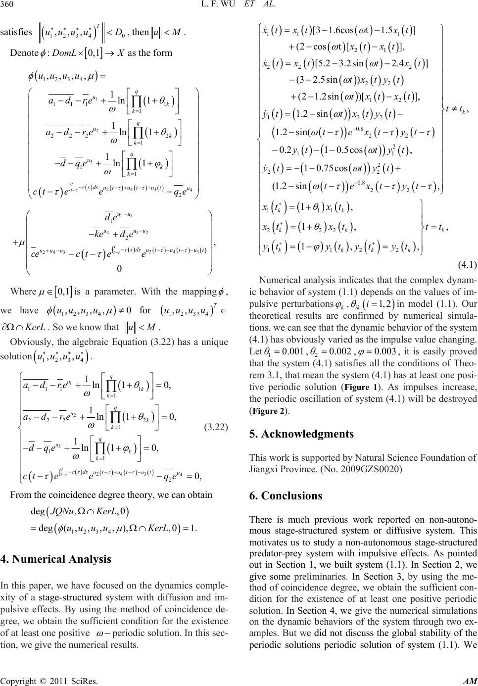

L. F. WU ET AL. 360
satisfies

1234 0
,,,T uuuu D
 , thenuM.
Denote


:0,1DomL X  as the form





 
1
2
3
243 4
1234
111 1
1
222 2
1
11
2
,,,,
1ln 1
1ln 1
1ln 1
t
t
q
uk
k
q
uk
k
q
uk
k
rsds ut ututu
uuuu
adre
adre
dqe
ct eeqe














 




 







 






 











  
21
412
243
243
1
2,
0
t
t
uu
uuu
rsds ut ut ut
uuu
de
ked e
cec tee








 


 





Where


0, 1  is a parameter. With the mapping

,
we have

1234
,,,, 0uuuu



for

1234
,,, T uuuu

K
erL. So we know that uM.
Obviously, the algebraic Equation (3.22) has a unique
solution

1234
,,,uuuu

.




  
1
2
3
2434
111 1
1
222 2
1
11
2
1ln 10,
1ln 10,
1ln 10,
0,
t
t
q
uk
k
q
uk
k
q
uk
k
rsds ut ut utu
adre
adre
dqe
ct eeqe













 


 




 




  








(3.22)
From the coincidence degree theory, we can obtain


1234
deg ,,0
deg(,,,,),,0 1.
JQNuKerL
uuuu KerL 


4. Numerical Analysis
In this paper, we have focused on the dynamics comple-
xity of a stage-structured system with diffusion and im-
pulsive effects. By using the method of coincidence de-
gree, we obtain the sufficient condition for the existence
of at least one positive

periodic solution. In this sec-
tion, we give the numerical results.

 
 
 
 
 

 



   

11 1
21
22 2
22
12
122
0.8 22
2
11
2
[3 1.6cost1.5]
(2cost [],
[5.2 3.2sin2.4]
(3 2.5sin)
(2 1.2sin)[],
1.2 sin
1.2 sin(
0.210.5cos,
10.75
xt xtxt
xt xt
xt xttxt
txtyt
txt xt
ytt xtyt
textyt
ytty t
yt









 
 
 

 
 
 

 




  
  




 

 


2
2
0.8 22
111
222
1122
,
cos
(1.2 sin,
1,
1, ,
1, ,
k
kk
kkk
kkkk
tt
tyt
textyt
xt xt
xtxttt
ytyt ytyt






























 


 

 





(4.1)
Numerical analysis indicates that the complex dynam-
ic behavior of system (1.1) depends on the values of im-
pulsive perturbationsk

,


1, 2
ik i
 in model (1.1). Our
theoretical results are confirmed by numerical simula-
tions. we can see that the dynamic behavior of the system
(4.1) has obviously varied as the impulse value changing.
Let 10.001


,20.002


,0.003

, it is easily proved
that the system (4.1) satisfies all the conditions of Theo-
rem 3.1, that mean the system (4.1) has at least one posi-
tive periodic solution (Figure 1). As impulses increase,
the periodic oscillation of system (4.1) will be destroyed
(Figure 2).
5. Acknowledgments
This work is supported by Natural Science Foundation of
Jiangxi Province. (No. 2009GZS0020)
6. Conclusions
There is much previous work reported on non-autono-
mous stage-structured system or diffusive system. This
motivates us to study a non-autonomous stage-structured
predator-prey system with impulsive effects. As pointed
out in Section 1, we built system (1.1). In Section 2, we
give some preliminaries. In Section 3, by using the me-
thod of coincidence degree, we obtain the sufficient con-
dition for the existence of at least one positive periodic
solution. In Section 4, we give the numerical simulations
on the dynamic behaviors of the system through two ex-
amples. But we did not discuss the global stability of the
periodic solutions periodic solution of system (1.1). We

L. F. WU ET AL. 361
Figure 1. Dynamic behavior of the system (4.1) with initial
values


1.2,1.2,0.8,0.6 ,=0.1τand impulsive perturbations
1=0.001θ,2= 0.002θ,= 0.003φ.
Figure 2. Dynamic behavior of the system (4.1) with initial
values


1.2,1.2,0.8,0.6 ,=0.1τand impulsive perturbations
1=0.1θ,2=0.2θ,=0.3φ.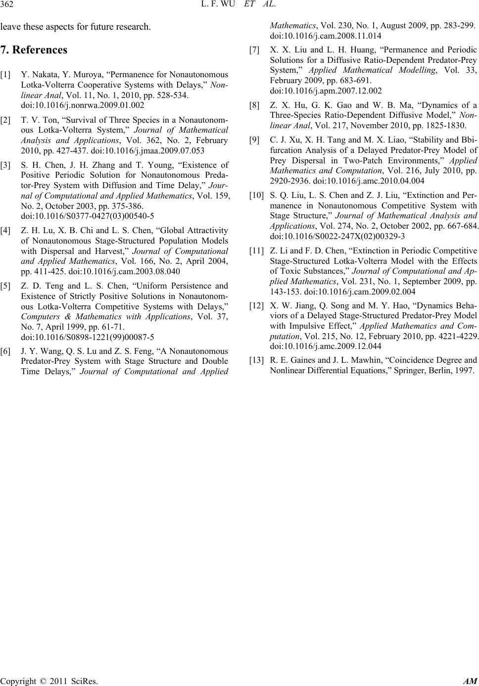

L. F. WU ET AL. 362
leave these aspects for future research.
7. References
[1] Y. Nakata, Y. Muroya, “Permanence for Nonautonomous
Lotka-Volterra Cooperative Systems with Delays,” Non-
linear Anal, Vol. 11, No. 1, 2010, pp. 528-534.
doi:10.1016/j.nonrwa.2009.01.002
[2] T. V. Ton, “Survival of Three Species in a Nonautonom-
ous Lotka-Volterra System,” Journal of Mathematical
Analysis and Applications, Vol. 362, No. 2, February
2010, pp. 427-437. doi:10.1016/j.jmaa.2009.07.053
[3] S. H. Chen, J. H. Zhang and T. Young, “Existence of
Positive Periodic Solution for Nonautonomous Preda-
tor-Prey System with Diffusion and Time Delay,” Jour-
nal of Computational and Applied Mathematics, Vol. 159,
No. 2, October 2003, pp. 375-386.
doi:10.1016/S0377-0427(03)00540-5
[4] Z. H. Lu, X. B. Chi and L. S. Chen, “Global Attractivity
of Nonautonomous Stage-Structured Population Models
with Dispersal and Harvest,” Journal of Computational
and Applied Mathematics, Vol. 166, No. 2, April 2004,
pp. 411-425. doi:10.1016/j.cam.2003.08.040
[5] Z. D. Teng and L. S. Chen, “Uniform Persistence and
Existence of Strictly Positive Solutions in Nonautonom-
ous Lotka-Volterra Competitive Systems with Delays,”
Computers & Mathematics with Applications, Vol. 37,
No. 7, April 1999, pp. 61-71.
doi:10.1016/S0898-1221(99)00087-5
[6] J. Y. Wang, Q. S. Lu and Z. S. Feng, “A Nonautonomous
Predator-Prey System with Stage Structure and Double
Time Delays,” Journal of Computational and Applied
Mathematics, Vol. 230, No. 1, August 2009, pp. 283-299.
doi:10.1016/j.cam.2008.11.014
[7] X. X. Liu and L. H. Huang, “Permanence and Periodic
Solutions for a Diffusive Ratio-Dependent Predator-Prey
System,” Applied Mathematical Modelling, Vol. 33,
February 2009, pp. 683-691.
doi:10.1016/j.apm.2007.12.002
[8] Z. X. Hu, G. K. Gao and W. B. Ma, “Dynamics of a
Three-Species Ratio-Dependent Diffusive Model,” Non-
linear Anal, Vol. 217, November 2010, pp. 1825-1830.
[9] C. J. Xu, X. H. Tang and M. X. Liao, “Stability and Bbi-
furcation Analysis of a Delayed Predator-Prey Model of
Prey Dispersal in Two-Patch Environments,” Applied
Mathematics and Computation, Vol. 216, July 2010, pp.
2920-2936. doi:10.1016/j.amc.2010.04.004
[10] S. Q. Liu, L. S. Chen and Z. J. Liu, “Extinction and Per-
manence in Nonautonomous Competitive System with
Stage Structure,” Journal of Mathematical Analysis and
Applications, Vol. 274, No. 2, October 2002, pp. 667-684.
doi:10.1016/S0022-247X(02)00329-3
[11] Z. Li and F. D. Chen, “Extinction in Periodic Competitive
Stage-Structured Lotka-Volterra Model with the Effects
of Toxic Substances,” Journal of Computational and Ap-
plied Mathematics, Vol. 231, No. 1, September 2009, pp.
143-153. doi:10.1016/j.cam.2009.02.004
[12] X. W. Jiang, Q. Song and M. Y. Hao, “Dynamics Beha-
viors of a Delayed Stage-Structured Predator-Prey Model
with Impulsive Effect,” Applied Mathematics and Com-
putation, Vol. 215, No. 12, February 2010, pp. 4221-4229.
doi:10.1016/j.amc.2009.12.044
[13] R. E. Gaines and J. L. Mawhin, “Coincidence Degree and
Nonlinear Differential Equations,” Springer, Berlin, 1997.