Applied Mathematics, 2011, 2, 271-282
doi:10.4236/am.2011.23032 Published Online March 2011 (http://www.SciRP.org/journal/am)
Effect of Point Source, Self-Reinforcement and
Heterogeneity on the Propagation of Magnetoelastic
Shear Wave
Amares Chattopadhyay, Shishir Gupta, Abhishek K. Singh, Sanjeev A. Sahu
Department of Applied Mathe mat i cs, Indian Scho ol of Mines, Dhanbad, In di a
Received October 1, 2010; revised November 1, 2010; accepted November 5, 2010
Abstract
This paper investigates the propagation of horizontally polarised shear waves due to a point source in a mag-
netoelastic self-reinforced layer lying over a heterogeneous self-reinforced half-space. The heterogeneity is
caused by consideration of quadratic variation in rigidity. The methodology employed combines an efficient
derivation for Green’s functions based on algebraic transformations with the perturbation approach. Disper-
sion equation has been obtained in the closed form. The dispersion curves are compared for different values
of magnetoelastic coupling parameters and inhomogeneity parameters. Also, the comparative study is being
made through graphs to find the effect of reinforcement over the reinforced-free case on the phase velocity.
It is observed that the dispersion equation is in assertion with the classical Love-type wave equation in the
absence of reinforcement, magnetic field and heterogeneity. Moreover, some important peculiarities have
been observed in graphs.
Keywords: Shear Wave, Magnetoelastic, Self-reinforcement, Dispersion Equation, Seismic Wave
1. Introduction
The study of mechanical behaviour of a self-reinforced
material has great importance in Geomechanics. Many
elastic fibre-reinforced composite materials are strongly
anisotropic in behaviour. It is desirable to study the shear
wave propagation in anisotropic media, as the propaga-
tion of elastic waves in anisotropic media is fundamen-
tally different from their propagation in isotropic media.
As the earth’s crust and mantle are not homogeneous, it
is also interesting to know the propagation pattern of
shear waves due to point source in heterogeneous me-
dium. The characteristic property of a self-reinforced
material is that its components act together as a single
anisotropic unit as long as they remain in elastic condi-
tion (i.e. the two components are bound together so that
there is no relative displacement between them). Self-
reinforced materials are a family of composite materials,
where the polymer fibres are reinforced by highly orien-
ted polymer fibres, derived from the same fibre. Alumina
or concrete is an example of self-reinforced material.
Under certain temperature and pressure some fibre mate-
rials may also be modified to self-reinforced materials by
reinforcing a matrix material of the same fibre. In real
life the fibres might be carbon, nylon, or conceivably
metal whiskers. It has been observed that the propagation
of elastic surface waves is affected by the elastic proper-
ties of the medium, through which they travel (Achen-
bach [1]). The Earth’s crust contains some hard and soft
rocks or materials that may exhibit self-reinforcement
property, and inhomogeneity is trivial characteristic of
the Earth. These facts motivate us towards this study.
The idea of introducing a continuous reinforcement at
every point of an elastic so lid was given by Belfield et al.
[2]. Later Verma and Rana [3] applied this model to the
rotation of tube, illustrating its utility in strengthening the
lateral surface of the tube. Verma [4] also discussed the
propagation of magnetoelastic shear waves in self-rein-
forced bodies. The problem of magnetoelastic transverse
surface waves in self-reinforced elastic solids was stu-
died by Verma et al. [5]. Chattopadhyay and Chaudhury
[6] studied the propagation, reflection and transmission
of magnetoelastic shear waves in a self-reinforced elastic
medium. Chattopadhyay and Chaudhury [7] studied the
propagation of magnetoelastic shear waves in an infinite
self-reinforced plate. Chattopadhyay and Venkateswarlu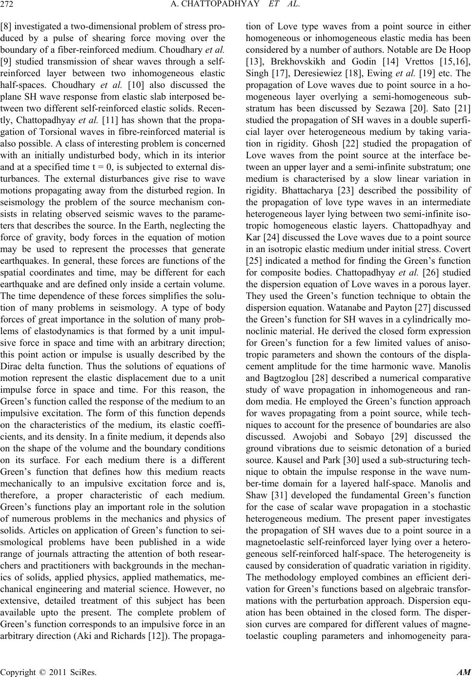

A. CHATTOPADHYAY ET AL. 272
[8] investigated a two-dimensional problem of stress pro-
duced by a pulse of shearing force moving over the
boundary of a fiber-reinforced medium. Choudhary et al.
[9] studied transmission of shear waves through a self-
reinforced layer between two inhomogeneous elastic
half-spaces. Choudhary et al. [10] also discussed the
plane SH wave response from elastic slab interposed be-
tween two different self-reinforced elastic solids. Recen-
tly, Chattopadhyay et al. [11] has shown that the propa-
gation of Torsional waves in fibre-reinforced material is
also possible. A class of interesting problem is concerned
with an initially undisturbed body, which in its interior
and at a specified time t = 0, is subjected to external dis-
turbances. The external disturbances give rise to wave
motions propagating away from the disturbed region. In
seismology the problem of the source mechanism con-
sists in relating observed seismic waves to the parame-
ters that describes the source. In the Earth, neglecting the
force of gravity, body forces in the equation of motion
may be used to represent the processes that generate
earthquakes. In general, these forces are functions of the
spatial coordinates and time, may be different for each
earthquake and are defined only inside a certain volume.
The time dependence of these forces simplifies the solu-
tion of many problems in seismology. A type of body
forces of great importance in the solution of many prob-
lems of elastodynamics is that formed by a unit impul-
sive force in space and time with an arbitrary direction;
this point action or impulse is usually described by the
Dirac delta function. Thus the solutions of equations of
motion represent the elastic displacement due to a unit
impulse force in space and time. For this reason, the
Green’s function called the response of the medium to an
impulsive excitation. The form of this function depends
on the characteristics of the medium, its elastic coeffi-
cients, and its density. In a finite medium, it depends also
on the shape of the volume and the boundary conditions
on its surface. For each medium there is a different
Green’s function that defines how this medium reacts
mechanically to an impulsive excitation force and is,
therefore, a proper characteristic of each medium.
Green’s functions play an important role in the solution
of numerous problems in the mechanics and physics of
solids. Articles on app lication of Green’s function to sei-
smological problems have been published in a wide
range of journals attracting the attention of both resear-
chers and practitioners with backgrounds in the mechan-
ics of solids, applied physics, applied mathematics, me-
chanical engineering and material science. However, no
extensive, detailed treatment of this subject has been
available upto the present. The complete problem of
Green’s function corresponds to an impulsive force in an
arbitrary direction (Aki and Richards [12]). The propaga-
tion of Love type waves from a point source in either
homogeneous or inhomogeneous elastic media has been
considered b y a number o f author s. Notab le are De Hoop
[13], Brekhovskikh and Godin [14] Vrettos [15,16],
Singh [17], Deresiewiez [18], Ewing et al. [19] etc. The
propagation of Love waves due to point source in a ho-
mogeneous layer overlying a semi-homogeneous sub-
stratum has been discussed by Sezawa [20]. Sato [21]
studied the propagation of SH waves in a double superfi-
cial layer over heterogeneous medium by taking varia-
tion in rigidity. Ghosh [22] studied the propagation of
Love waves from the point source at the interface be-
tween an upper layer and a semi-infinite substratum; one
medium is characterised by a slow linear variation in
rigidity. Bhattacharya [23] described the possibility of
the propagation of love type waves in an intermediate
heterogeneous layer lying between two semi-infinite iso-
tropic homogeneous elastic layers. Chattopadhyay and
Kar [24] discussed the Love waves due to a point source
in an isotrop ic elastic medium under initial stress. Covert
[25] indicated a method for finding the Green’s function
for composite bodies. Chattopadhyay et al. [26] studied
the dispersion equation of Love waves in a porous layer.
They used the Green’s function technique to obtain the
dispersion equ at i on. Wat a nabe and Payton [27] discussed
the Green’s function for SH waves in a cylindrically mo-
noclinic material. He derived the closed form expression
for Green’s function for a few limited values of aniso-
tropic parameters and shown the contours of the displa-
cement amplitude for the time harmonic wave. Manolis
and Bagtzoglou [28] described a numerical comparative
study of wave propagation in inhomogeneous and ran-
dom media. He employed the Green’s function approach
for waves propagating from a point source, while tech-
niques to account for the presence of boundaries are also
discussed. Awojobi and Sobayo [29] discussed the
ground vibrations due to seismic detonation of a buried
source. Kausel and Park [30] used a sub-structu ring tech-
nique to obtain the impulse response in the wave num-
ber-time domain for a layered half-space. Manolis and
Shaw [31] developed the fundamental Green’s function
for the case of scalar wave propagation in a stochastic
heterogeneous medium. The present paper investigates
the propagation of SH waves due to a point source in a
magnetoelastic self-reinforced layer lying over a hetero-
geneous self-reinforced half-space. The heterogeneity is
caused by consideration of quadratic variation in rigidity.
The methodology employed combines an efficient deri-
vation for Green’s functions based on algebraic transfor-
mations with the perturbation approach. Dispersion equ-
ation has been obtained in the closed form. The disper-
sion curves are compared for different values of magne-
toelastic coupling parameters and inhomogeneity para-

A. CHATTOPADHYAY ET AL. 273
meters. Also, the comparative study is being made throu-
gh graphs to find the effect of reinforcement over the
reinforced-free case on the phase velocity. It is observed
that the dispersion equation is in assertion with the clas-
sical Love-type wave equation in the absence of rein-
forcement, magnetic field and heterogeneity.
2. Formulation and Solution of the Problem
We have considered a magnetoelastic self-reinforced
layer of thickness
H
lying over a heterogeneous self-
reinforced half-space. The x-axis has been taken along
the propagation of waves and z-ax is is positive vertically
downwards as shown in Figure 1. The source of distur-
bance S is taken at the point of intersection of the inter-
face of separation and z-axis. At first, we need to find the
equation governing the propagation of SH wave in self
reinforced magnetoelastic crustal layer.
The constitutive equations used in a self-reinforced li-
nearly elastic model are (Belfield et al. 1983)

 
*
*
2
2
,,, 1,2,3
ijkkijT ijkm kmijkkij
L
Tikkjjkkikmkmi j
eeaaeeaa
aaeaaeaa eaa
ijkm
 
 
 
 

(1)
where ij

are components of stress, ij e components of
infinitesimal strain, ij

Kronecker delta, i acomponents
of a
, all referred to rectangular cartesian co-ordinates

123
,,
i
x
aaaa
 is the preferred directions of reinfor-
cement such that 222
123
1aaa. The vector a

may
be function of position. Indices take the values 1, 2, 3
and summation convention is employed. The coefficients
**
,,,
T

 and

2
L
T

  are elastic constants with
dimension of stress. T

can be identified as the shear
modulus in transverse shear across the preferred direc-
tion, and
L

as the shear modulus in longitudinal shear
in the preferred direction. *

and *

are specific stress
components to take into account different layers for con-
crete part of the composite material. The model consi-
dered here is of transversely isotropic material, also
z
= 0
z
=
H
Figure 1. Geometry of the problem.
known as materials of hexagonal symmetry.
Equations governing the propagation of small elastic
disturbances in a perfectly conducting self-reinforced
elastic medium having electromagnetic force
J
B



(the Lorentz force,
J

 being the electric current density
and B

 being the magnetic induction vector) as the only
body force are

2
,2i ij ji
u
JB t


 

 (2)
where


i
J
B

 is the i
x
-component of the force


J
B



and

is the density of the layer. Here inte-
raction of mechanical and electromagnetic fields is con-
sidered.
Let


11 1
,,
i
uuvw and denoting 12 ,,
x
xx y
3
x
z

th en Equation (2) can be written as



2
13 11 121
2
2
23 12 221
2
2
13 23 331
2
x
y
z
u
JB
xyz t
v
JB
xyz t
w
JB
xyz t
  
  
 
 
 


 


  


 


 


 





(3)
For SH wave propagating in the x-direction and caus-
ing displacement in the y-direction only, we shall assume
that


11 11
0,, ,uw vvxzt and 0.
y

 (4)
Using Equation (4) in Equation (3), we have

2
23
12 1
2
y
v
JB
xz t
  



 

 (5)
where

111
121 13TLT
vvv
aa a
x
xz
 








111
233 13TLT
vvv
aa a
zxz
 








For stresses 12

and 23

, the first part indicate the
shear stress due to elastic members (steel) and the second
part indicates effect of comparatively non-elastic mate-
rial of the composite section in the same direction.
The first component would be having the term T

,
which can be termed as elastic coefficient and


L
T

  in the second term amounts for the effect
comparatively non-elastic portion of the composite ma-
terial.
The well known Maxwell’s equations governing the
electromagnetic field are

A. CHATTOPADHYAY ET AL. 274
0,, ,
and .
i
e
B
BE HJ
t
u
BH JEB
t



 













  
  
(6)
where E
 is the induced electric field,
J
 is the current
density vector and magnetic field
H
 includes both pri-
mary and induced magnetic fields. e

and

are the
induced permeability and conduction coefficient respec-
tively.
The linearized Maxwell’s stress tensor

0x
M
ij
 due to
the magnetic field is given by


0x
M
ijeijj ik kij
HbHb Hb

 .
Let

,,
x
yz
H
HH H
 and

123
,, .
i
bbbbi b is the
change in the magnetic field. In writing the above equa-
tions, we have neglected the displacement current.
From Equation (6), we get
2. i
e
u
H
HH
tt





 



 


 (7)
In component form, Equation (7) can be written as
2
2
11
2
1,
1,
1
and .
xx
e
zz
e
xz
yy
e
HH
t
HH
t
vv
HH
Htt
H
txz













 











 



(8)
For perfectly conducting medium, (i.e.

), it
can be seen that Equations (8) become
0,
xz
HH
tt


 (9)
and
11
.
xz
y
vv
HH
Htt
tx z







 
(10)
Assuming that primary magnetic field is uniform
throughout the space. It is clear from Equation (10) that
there is no perturbation in
x
H
and
z
H
, however from
Equation (10) there may be perturbation in
y
H
. There-
fore, taking small perturbation, say 2 b in
y
H
, we have
0102 2
,
xy
H
HH Hb and 03,
Z
H
Hwhere

01 0203
,,HHH are components of the initial magnetic
field 0
H
.
We can write


00 0
cos ,0,sinHH H

 

, where
00
H
H

 and

is the angle at which the wave
crosses the magnetic fiel d. Thus we have


020
cos ,,sinHH bH

 

 (11)
We shall consider initial value of 2
bto be zero. Using
Equation (11) in Equation (10), we get
11
00
2
cos sin
.
vv
HH
btt
tx z








 
(12)
Integrating with respect to t, we get
11
20 0
cossin .
vv
bH H
x
z





 (13)
Considering

2.
2
H
H
HHH





  and
the Equations (6), we get

2.
2
eH
J
BHH 





 

 





  (14)
Using the Equations (1) and (14), we obtain the equa-
tion of the motion for the magnetoelastic self-reinforced
layer as
  
2222
111
1111
222
,
vvvv
PQR
xz
zx t


 


(15)
where






1222
30
1222
10
12
13 0
sin ,
cos
and2sin 2.
TLTe
TLTe
LT e
Pa H
Qa H
Raa H



 




 




(16)
If


1,rt
 be the force density distribution in the
upper layer due to the point source, the equation of mo-
tion for SH wave propagation along x-axis becomes as



 



11 2222
1
1111
22 2
11 11
4,rt
vvv v
QR
xz
zx t
PPP P



 

 (17)
where r is the distance from the origin, where the force
is applied to a point of coordinates and t is the time.
Considering


11
,,, it vxzt Vxze

 and




11
,it rt re

  in Equation (17), we obtain



 



11
222 21
111
1
22 111 1
4r
VVV QR V
xz zx
PP PP

 

  (18)
where kc


is the angular frequency, k the wave
number and c is the phase velocity. Here the distur-
bances caused by the impulsive force

1r
 may be
represented in terms of Dirac-delta function at the so urce

A. CHATTOPADHYAY ET AL. 275
point as

1rxzH
 
Therefore the equation of motion for the upper magne-
toelastic self-reinforced layer with an impulsive point
source is



 





11
222
2
111
1
22 11 11
4
x
zH
VVV QR V
xz zx
PP PP
 




 
(19)
Defining the Fourier transform

,
r
Vz  of


,
r
vxz
as
 
1
,,
2
ix
rr
Vz vxzedx




 (20)
Then the inverse transform can be given as
 
1
,,
2
ix
rr
vxzVze d





 (21)
Now taking the Fourier transform of Equation (19), we
obtain




22
11
111 1
21
24 zH
dV dV
f
rV z
dz dz P
 
 (22)
where

 


11
2
22
11
111
,
RQ
fi r
PPP



The heterogeneity of the lower inhomogeneous self-
reinforced elastic half-space has been considered in the
form
 

 

2
20
2
20
LL
TT
zH
zH



 (23)
Now, the equation of motion for the lower heteroge-
neous self-reinforced elastic half-space is
  

222 2
222
222 22
0
22 2
2
vvv vv
PQR zH
xz z zx t

 
 
  
(24)
where 0

is the density of the lower half-space,
 




 

22 22
2
3
22 22
2
1
222
13
,
and 2.
TLT
TLT
LT
Pa
Qa
Raa



 
 

In view of substitution


22
,,, it vxztVxze

 and
Equation (20), Equation (24) becomes

22
21
2222
24
dV dV
f
rV z
dz dz
  (25)
where

 


22
2
22 000
22
222
000
,
RQ
fir
PPP






 
2
2
22
2 21 2
2
2
0
4
2
z
dV dV
zHzHzH V
dz
dz
P





 



(26)
 


 

 

2
20 00
2
03
000
2
01
200
013
,
and 2
TLT
TLT
LT
Pa
Qa
Raa



 
 

Now it is clear from Equation (25) that the displace-
ment in the lower medium may be determined by assu-
ming the lower medium to be homogeneous, isotropic
having source density distribution

2z
 .
Substituting

2
r
z
f
rr
Vz Vze


in Equation (22) and
Equation (25) for 1, 2r

respectively, we obtain

22
11
11
242
dV fz
Vze
dz


 (27)
and

22
22
22
242
dV fz
Vze
dz


 (28)
where
22
2222 12
12
,
44
ff
rr 


The boundary conditions are

111
10, at0
2
dV f
PVz
dz




 (29)
12
,atVV zH

 (30)
  12
112 2
12
,at
22
dV fdVf
PVP VzH
dz dz
 

 
 
  (31)
Thus Equations (27) and (28) together with prescribed
boundary conditions (29) to (31) give the complete ma-
thematical model for the p roblem. Now we apply Green’s
function technique to solve it. If

10
Gzzis the Green’s
function for the upper layer satisfying the condition
10
dG
dz

at 0z

and at zH, then the equation sa-
tisfied by


10
Gzz is

 
210 2
1100
2
dG zzGzz zz
dz
  (32)
where 0 z is a point in the upper medium and z is the
field point. Multiplying the Equation (27) by


10
Gzz

A. CHATTOPADHYAY ET AL. 276
and Equation (32) by

1
Vz
, then subtracting and inte-
grating with respect to z from 0z to zH

, we
have



1
12
10 1010
1
2fH
zH
dV
GHzeGHzV z
dz P

  


 (33)
Since

10
0
dGz z
dz  at 0z and zH.
Replacing 0 z by zand remembering that




11
GHz GzH, the Equation (33) gives the value
of 1
V

at any point z in the upper medium as



11
2
111
1
2fH
z
H
dV
VzeGzH GzHdz
P

 



Therefore,



 
111
2
1111
1
2
2
fzH
zH
dV zf
VzeGzHGzHVz
dz
P












(34)
Now, let

20
Gzz be the Green’s function for the
lower medium, as per previous discussion may be as-
sumed to be homogeneous. We assume that


20
Gzz
is the solution of the equation
  
220 2
1200
2
dG zzGzz zz
dz
  (35)
where 0 z is the point in the lower medium, satisfying
the condition 20
dG
dz  at zH

and approaches to
zero as z . Multiplying Equation (28) by


20
Gzz and Equation (35) by

2
Vz
, then subtract-
ing and integrating with respect to z from zH

to
z

, we have
   
2
22
2022020
/4
fz
H
zH
dV
GHzezGzzdzVz
dz




 
 

 
(36)
Interchanging z by 0
z in the Equation (36), the
value of


2
Vz

at an y point z in the lower medium is
   
20
22
22 20200
4fz
H
zH
dV
Vz GzHezGzzdz
dz







 
Therefore,
     
20
22 22
22 2
222 20200
/4
2
fz fz fH
H
zH
dV zf
Vzee GzHVzezGzzdz
dz














 (37)
With the help of bound ary condition (30), we have



 


 
20 2
12
12
22
111 222020
1
24/
22
fz fH
H
zH zH
dV zdVz
ff
GHH GHHVzGHHVzeezGzzdz
dz dz
P




 
 
 
 
 
 

(38)
Using boundary condition (31), Equation (38) can be written as
 


 
20 2
1122
12 20200
1
10
12 4
2
fz fH
H
zH
dV zfVzGHHeezGHzdz
dzD P





 
 
 
 





 (39)
where 1 D is given in appendix I.
Substituting the value of
 
111
2
z
H
dV zfVz
dz







from
Equation (39) and


20
4z  from Equation (26) into
Equation (34), we obtain












   
2
1
22
20
2
12 1
2
111
01 201 2
2
22
2 22 2
00020200
20
0
2
2
fH
fzH
fz
H
GzHGHHe GzH
Vz ePGHHP GHHPGHHP GHH
dV dV
zHzH zHVzeGHzdz
dz dz





















(40)

A. CHATTOPADHYAY ET AL. 277
In view of boundary condition (31), relation (37) gives









 




 


2
2
222
20
2
2
1
2
12 2
2
211
012 001 2
2
22
2
22 2
00020200
20
0
2
222
2
22
00020
20
0
0
2/ //
// //
2/
2
fz
fzH
fz
H
fz
GHHGzHe GzHP
Vz ePGHH PGHHPPGHHPGHH
dV dV
zHzH zHVzeGHzdz
dz
dz
dV dV
ezHzH zHVz
dz dz
P

























20
2200
/
fz
H
eGzzdz





 



(41)

2
Vzcan be obtained from the relation (41) by the
method of successive approximations. The value of

2
Vz obtained from Equation (41) when substituted in
Equation (40) gives the value of

1
Vz. We are interes-
ted in the value of

1
Vz, which will give the displace-
ment in the upper layer, and since the higher order of

can be neglected; we ta ke as th e fi rst order ap pro ximation
 





2
2
2
12
21
01 2
2fzH GHHGzHe
Vz PGHHP GHH

 (42)
which gives the displacement at any point in the lower
medium if it is taken as homogeneous. Putting this value
of


2
Vzin Equation (40), we get
 












 
 
11
22
22
12 11
12
11
012 01 2
2
2 2
20
20 2
2
00020200
20
0
22
2
ff
zH zH
H
GzHGHHee GzHGHH
Vz PGHHP GHHPGHHPGHH
dGz H
dGz H
zH zH zHGzHGHzdz
dz
dz


 





 




(43)
The solution of Equation (43) represents the elastic
displacements due to a unit impulse force in space and
time. Thus the Green’s function is the response of the
medium to an impulsive excitation. If we know the val-
ues of

1
GzH and

2
GzH, then the value of

1
Vz
can be determined from the Equation (43). We
have assumed

10
Gzz as the solution of Equation
(32). A solution of Equation (32) may also be ob tained in
the following manner.
We have the equation
22
20.
d
dz

 (44)
Two independent solutions of Equation (44), vanish-
ing at z and z are

1
z
ze

 and

2
z
ze


.
Therefore the solution of th e Equation (44) for an infi-
nite medium is
 
120
zz
W
 for 0,zz




10 2
zz
W
 for 0,zz
where
 
121 220.Wzz zz




So, the solution of Equation (32) is 0.
2
zz
e




Since


10
Gzzis to satisfy the cond ition
10
dG
dz

at 0z

and zH (45)
Therefore, we can assume that

0
10 12.
2
zz
zz
e
GzzCeCe





 
where 12 andCCare the arbitrary constants which can be
evaluated using condition (45). We finally get











00 00
0
101.
2
Hz HzHz Hz
zz
zz
HH HH
eeee ee
Gzz eee ee
 




  






 




(46)
Therefore,

A. CHATTOPADHYAY ET AL. 278

11,
zz
HH
ee
GzH ee







 


(47)

11,
HH
HH
ee
GHH ee







 


(48)
Similarly, the value of


20
/Gzz can be written as


00
2
20 1,
2
zzzz H
Gzze e


 


 

 (49)
and so


0
20
z
H
e
GHz



 (50)

21.GHH

 (51)
Substituting all these values in Equation (43), we get













1
22
2
22
111
00
1
214
fHH
zH zz
HH HHHHHH
ee
eee
Vz Pee PeePeePee


  


  

 
 







 





  






(52)
Neglecting the higher powers of

the Equation (52) may be approximated as






 





1
2
2
2
12
2
1
01
0
2
1
14
fzHzz
HH
HH HH
HH HH
eee
Vz
ee
Pee PeePee Pee


 
 


  
 










 



 


 






(53)
Taking the inverse Fourier transform of Equation (53), the displacement in the upper medium may be obtained as






 





1
2
2
2
12
2
1
01
0
2
1
14
fzHzzix
HH
HH HH
HH HH
eeeed
Vz
ee
Pee PeePee Pee


 
 



  
 

 














 


 






 (54)
The dispersion equation of SH waves will be obtained by equating to zero the denominator of the above in tegral, i.e.



 





2
2
2
2
1
01
0
1
10.
4
HH
HH HH
HH HH
ee
Pee PeePee Pee

 
 



 










 

 



(55)
In view of the substitutions 12 andik k

  the
above Equation (55) gives the dispersion relation of shear waves in magnetoelastic self-reinforced layer lying over hetero geneous self-reinforced hal f -space


  









2
22
02
111 22
222 22
0
112 22
00 00
32
22022
00 00
1
tan 1.
411
22
L
T
c
P
kH PkPQR QR
a
PP PP


 








 

 

  



 


  


  
 

 

(56)
where

A. CHATTOPADHYAY ET AL. 279
121 2
,and

  are given in the appendix I.
3. Particular Cases
3.1. Case I
When 0

 the dispersion relation (56) reduces to



2
02
111
tan P kH P



.
which is the dispersion equation of shear waves for the
case of magnetoelastic self-reinforced layer lying over a
homogeneous self-reinforced half-space due to a point
source.
3.2. Case II
When
  00
12
0, and
LTL T

   the dis-
persion relation (56) reduces to



1/2
2
22
3
1/2
2
22
4
1/2
2
2
122
3
tan 1
1sin
1
1sin 1
1sin
H
H
H
c
kH
c
c
 

 
 


















where
34
,and
H

 are given in the appendix I.
which is the dispersion equation of shear waves for the
case of isotropic magnetoelastic layer lying over a ho-
mogeneous isotropic half-space due to a point source.
3.3. Case III
When
 
00
12
0, 0,and
HLT LT

  
the dispersion relation (56) reduces to
1/2
2
1/2 22
24
21/2
2
3
12
3
1
tan 1
1
c
c
kH c






 


 
 


which is the classical Love wave equation.
4. Numerical Examples
For the case of a magnetoelastic self-reinforced layer
lying over a non-homogeneous self-reinforced half space,
we take the following data
1) For Magnetoelastic Self-reinforced layer, [Mark-
ham [32]]
92 923
1
5.6610 N/m ,2.4610 N/m ,7,800Kg/m.
LT
  
2) For Heterogeneous Self-reinforced half space,
[Chattopadhyay and Chaudhur y [6]]
 
00
92 923
2
7.0710 N/m ,3.510 N/m ,1,600Kg/m.
LT
  
Moreover the following data are used (Hool and Kinne
[33]; Maugin [34])
2
10,0.00316227,0.0,0.05,0.1,0.0,0.25,0.5
HT
H
a

 
The effect of reinforcement, magnetic field and hete-
rogeneity on the propagation of plane SH waves in a
magnetoelastic self-reinforced layer lying over an hetero-
geneous self-reinforced half spaces has been depicted by
means of graphs. Figures 2 and 3 gives the variation of
non-dimensional phase velocity

1
c

with respect to
non-dimensional wave number kH for different values
of inhomogeneity



and magnetoelastic coupling
parameters


H

respectively. The small change in the
non-dimensional wave number produces substantial
change in non-dimensional phase velocity in both the
cases. In each of these figures graphs are drawn for both
in the presence and absence of reinforcement. In both the
figures solid line curve 1, 2 & 3 refers to the case of
reinforcement where as dotted line curves 4, 5 & 6 cor-
respond to the reinforced free case. The comparative stu-
dy of the graphs reveals that with the increase in hetero-
geneity and magnetoelastic coupling parameter, the phase
velocity increases for both reinforced and reinforced free
cases. It is important to add that the impact of reinforce-
ment is dominant on the reinforced free case.
00.5 11.5 22.5 3
1
1. 2
1. 4
1. 6
1. 8
2
2. 2
2. 4
kH
c/

1
1
23
456
1: a
1
=0.00316227,

=0.0
2: a
1
=0.00316227,

=0.25
3: a
1
=0.00316227,

=0.50
4: a
1
=a
3
=0.0,

=0.0
5: a
1
=a
3
=0.0,

=0.25
6: a
1
=a
3
=0.0,

=0.50
Figure 2. Dimensionless phase velocity against dimension-
less wave number for =0.0
H
ε in presence and absence
of reinforcement.
1: a1 = 0.00316227,

= 0.0
2: a1 = 0.00 316227 ,

= 0.25
3: a1 = 0.00316227,

= 0.50
4: a1 = a3 = 0.0,

= 0.0
5: a1 = a3 = 0.0,

= 0.25
6: a1 = a3 = 0.0,

= 0.50
kH
1
c


A. CHATTOPADHYAY ET AL. 280
00.5 11.5 22.5 3
1
1.2
1.4
1.6
1.8
2
2.2
2.4
kH
c/

1
1
2
3
4
5
6
1: a
1
=0.00316227,

H
=0.0
2: a
1
=0.00316227,

H
=0.05
3: a
1
=0.00316227,

H
=0.10
4: a
1
=a
3
=0.0,

H
=0.0
5: a
1
=a
3
=0.0,

H
=0.05
6: a
1
=a
3
=0.0,

H
=0.10
Figure 3. Dimensionless phase velocity against dimension-
less wave number for =0.0ε in presence and absence of
reinforcement.
In Figure 4 curve 1 stands for the isotropic homoge-
neous layer lying over isotropic homogeneous half space,
curve 2 stands for the isotropic magnetoelastic homoge-
neous layer lying over isotropic homogeneous half space,
curve 3 stands for isotropic magnetoelastic homogeneous
layer lying over isotropic heterogeneous half space,
curve 4 stands for the self-rein forced homogeneous layer
lying over a homogeneous self-reinforced half space,
curve 5 stands for the magnetoelatic self-reinforced ho-
mogeneous layer lying over a homogeneous self-reinfor-
ced half space and curve 6 stands for the magnetoelatic
self-reinforced homogeneous layer lying over a hetero-
geneous self-reinforced half space. The comparative stu-
dy shows that as anisotrop y prevails through self-r einfor-
cement, magnetoelasticity prevails through magnetoelas-
tic coupling parameter and heteroge neity prevails thro ugh
inhomogeneity parameter in the medium, the phase velo-
city of the SH waves due to a poin t sour ce gets suppor ted
more and more. It is also evident that the coupling para-
meters

H

and the heterogeneity



both support
the phase velocity but the effect of heterogeneity is pro-
minent.
5. Conclusions
Massive earth crust with built up RCC and Masonry in-
frastructures considerably influence the seismic waves
propagation mainly due to elast i c pr operties of the media.
The present study has established that the phase velocity
dispersion curve is affected by its magnetoelastic rein-
forced parameters and irregular boundaries. Ground sha-
king and earthquake loads can be visualized through this
study. It is the fact that the earth crust and built up RCC
and masonry structures over it will be proportiona tely af-
00.5 11.5 22.5 3
1
1. 2
1. 4
1. 6
1. 8
2
2. 2
2. 4
kH
c/

1
1
2
3
4
5
6
1: a
1
=a
3
=0.0,

=0.0,

H
=0.0
2: a
1
=a
3
=0.0,

=0.0,

H
=0.1
3: a
1
=a
3
=0.0,

=0.5,

H
=0.1
4: a
1
=0.00316227,

=0.0,

H
=0.0
5: a
1
=0.00316227,  =0.0, 
H
=0.1
6: a
1
=0.00316227,

=0.5,

H
=0.1
Figure 4. Dimensionless phase velocity against dimension-
less wave number for different cases.
fected by the response of the ground motion for these
wave propagation. RCC and masonr y structures hav e dy-
namic properties like mass, stiffness and strength respon-
sible for vibrati on parame ters due to grou nd motion. Seis-
mic forces are proportional to the mass of the structures
and the acceleration caused by the ground movement. Fre-
quency is the measure of how often ground motion chan-
ges direction. Am plitude is a m easure of the magni tude of
this motion. These parameters will be of great help for
foundatio n design capa ble of translat ion. A well -designed
and well-built RCC structure has a reliable load path that
transfers these disturbing forces through the structures to
the foundation where the soil can resist them.
Besides earthquake, the ground motion may be due to
heavy plant operation, blasting, rolling or falling of heavy
masses. All these may cause harmonically forced vibra-
tion or transi ent vibr ation with im pulse and ar bitrary exci-
tation to the reinforced media. For th ese conditio ns, there
are well established methods to calculate principal modes
of vibration and associated param eters. Wave propagation
phenomenon in reinforced media is one of the most im-
portant information for the design and development of
heavy civil co nstruction pr ojects. If the nat ure and source s
of ground movement are predictable, then the design of
RCC, masonry and steel structures for the construction of
buildings, towers and bridges will be more accurate, sci-
entific and safe.
The present study has established that increase in he-
terogeneity and magnetoelastic coupling parameter in-
creases the phase velocity for both reinforced and rein-
forced free cases. It is important to add that the impact of
reinforcement is dominant on the reinforced free case.
Hence the study of magnetoelastic shear wave propaga-
tion due to a point source in magnetoelastic self-reinfor-
ced layer over a heterogeneous self-reinforced half-space
1: a1 = 0.00316227,
H

= 0.0
2: a1 = 0.00 316227 ,
H

= 0.05
3: a1 = 0.00316227,
H

= 0.10
4: a1 = a3 = 0.0,
H

= 0.0
5: a1 = a3 = 0.0,
H

= 0.05
6: a1 = a3 = 0.0,
H

= 0.10
kH
1
c

kH
1: a1 = a3 = 0.0,

= 0.0,
H

= 0.0
2: a1 = a3 = 0.0,

= 0.0,
H

= 0.1
3: a1 == a3 = 0.0,

= 0.5,
H

= 0.1
4: a1 = 0.00316 227,

= 0.0,
H

= 0.0
5: a1 = 0.003 16227,

= 0.0,
H

= 0.1
6: a1 = 0.00316227,

= 0.5,
H

= 0.1
1
c


A. CHATTOPADHYAY ET AL. 281
provides valuable information for selection of proper
structural materials for present day construction work.
6. Acknowledgements
The authors convey their sincere thanks to Indian School
of Mines, Dhanbad for providing JRF to Mr. Abhishek
Kumar Singh and also facilitating us with its best facility.
Acknowledgement is also due to DST, New Delhi for the
providing financial support through Project No. SR/S4/
MS: 436/07, Project title: “Wave propagation in aniso-
tropic media”.
7. References
[1] J. D. Achenbach, “Wave Propagation in Elastic Solids,”
North Holland Publication Company, New York, 1975.
[2] A. J. Belfield, T. G. Rogers and A. J. M. Spencer, “Stress
in Elastic Plates Reinforced by Fibers Lying in Concen-
tric Circles,” Journal of the Mechanics and Physics of
Solids, Vol. 31, No. 1, 1983, pp. 25-54.
doi:10.1016/0022-5096(83)90018-2
[3] P. D. S. Verma and O. H. Rana, “Rotation of a Circular
Cylindrical Tube Reinforced by Fibres Lying along He-
lices,” Mechanics of Materials, Vol. 2, No. 4, 1983, pp.
353-359. doi:10.1016/0167-6636(83)90026-1
[4] P. D. S. Verma, “Magnetoelastic Shear Waves in Self-
Reinforced Bodies,” International Journal of Engineer-
ing Science, Vol. 24, No. 7, 1986, pp. 1067-1073.
doi:10.1016/0020-7225(86)90002-9
[5] P. D. S. Verma, O. H. Rana and M. Verma, “Magnetoe-
lastic Transverse Surface Waves in Self-Reinforced Elas-
tic Bodies,” Indian Journal of Pure and Applied Mathe-
matics, Vol. 19, No. 7, 1988, pp. 713-716.
[6] A. Chattopadhyay and S. Chaudhury, “Propagation, Ref-
lection and Transmission of Magnetoelastic Shear Waves
in a Self Reinforced Medium,” International Journal of
Engineering Science, Vol. 28, No. 6, 1990, pp. 485-495.
doi:10.1016/0020-7225(90)90051-J
[7] A. Chattopadhyay and S. Chaudhury, “Magnetoelastic
Shear Waves in an Infinite Self-Reinforced Plate,” Inter-
national Journal of Numerical and Analytical Methods in
Geomechanics, Vol. 19, No. 4, 1995, pp. 289-304.
doi:10.1002/nag.1610190405
[8] A. Chattopadhyay and R. L. K. Venkateswarlu, “Stre sses
Produced in a Fibre-Reinforced Half Space Due to Mov-
ing Load,” Bulletin of Calcutta Mathematical Society,
Vol. 90, 1998, pp. 337-342.
[9] S. Chaudhary, V. P. Kaushik and S. K. Tomar, “Trans-
mission of Shear Waves through a Self-Reinforced Layer
Sandwiched between Two Inhomogeneous Viscoelastic
Half-Spaces,” International Journal of Mechanical Scien-
ces, Vol. 47, No. 9, 2005, pp. 1455-1472.
doi:10.1016/j.ijmecsci.2005.04.011
[10] S. Chaudhary, V. P. Kaushik and S. K. Tomar, “Plane
SH-Wave Response from Elastic Slab Interposed be-
tween Two Different Self Reinforced Elastic Solids,” In-
ternational Journal of Applied Mechanics and Engineer-
ing, Vol. 11, No. 4, 2006, pp. 787-801.
[11] A. Chattopadhyay, S. Gupta, S. K. Samal and V. K.
Sharma, “Torsional Wave in Self-Reinforced Medium,”
International Journal of Geomechanics, Vol. 9, No. 1,
2009, pp. 9-13.
doi:10.1061/(ASCE)1532-3641(2009)9:1(9)
[12] K. Aki and P. G. Richards, “Quantitative Seismology:
Theory and Methods,” W. H. Freeman & Co., New York,
1980.
[13] A. T. De Hoop, “Handbook of Radiation and Scattering
of Waves: Acoustic Waves in Fluids, Elastic Waves in
Solids, Electromagnetic Waves,” Academic Press, Lon-
don, 1995.
[14] L. M. Brekhovskikh and O. A. Godin, “Acoustics of
Layered Media,” Springer-Verlag, Berlin, 1992.
[15] C. Vrettos, “Forced Anti-Plane Vibrations at the Surface
of an Inhomogeneous Half-Space,” Soil Dynamics and
Earthquake Engineering, Vol. 10, No. 5, 1991, pp. 230-
235. doi:10.1016/0267-7261(91)90016-S
[16] C. Vrettos, “The Boussinesq Problem for Soil with
Bound Nonhomogeneity,” International Journal of Nu-
merical and Analytical Methods in Geomechanics, Vol.
22, No. 8, 1998, pp. 655-669.
doi:10.1002/(SICI)1096-9853(199808)22:8<655::AID-N
AG938>3.0.CO;2-R
[17] K. Singh, “Love Waves Due to a Point Source in an
Axially Symmetric Heterogeneous Layer between Two
Homogeneous Half Spaces,” Pure and Applied Geophys-
ics, Vol. 72, No. 1, 1969, pp. 35-44.
doi:10.1007/BF00875690
[18] H. Deresiewich, “A Note on Love Waves in Homogene-
ous Crust Overlying an Inhomogeneous Substratum,”
Bulletin of Seismological Society of America, Vol. 52,
1962, pp. 639-645.
[19] M. Ewing, W. S. Jardetzky and F. Press, “Elastic Waves
in Layered Media,” McGraw-Hill, New York, 1957.
[20] K. Sezawa, “Love Waves Generated from a Source of a
Certain Depth,” Bulletin of the Eathquake Research In-
stitute, University of Tokyo, Vol. 13, 1935, pp. 1-17.
[21] Y. Sato, “Love Waves Propagated upon Heterogeneous
Medium,” Bulletin of the Eathquake Research Institute,
University of Tokyo, Vol. 30, 1952, pp. 1-12.
[22] M. L. Ghosh, “Love Wave Due to a Point Source in an
Inhomogeneous Medium,” Gerlands Beitrage Zur Geo-
physik, Vol. 70, 1970, pp. 319-342.
[23] J. Bhattacharya, “The Possibility of the Propagation of
Love Type Waves in an Intermediate Heterogeneous
Layer Lying between Two Semi-Infinite Isotropic Ho-
mogeneous Elastic Layers,” Pure and Applied Geophys-
ics, Vol. 72, No. 1, 1969, pp. 61-71.
doi:10.1007/BF00875693
[24] A. Chattopadhyay and B. K. Kar, “Love Wave Due to a
Point Source in an Isotropic Elastic Medium under Initial
Stress,” International Journal of Non-Linear Mechanics,
Vo. 16, No. 3-4, 1981, pp. 247-258.

A. CHATTOPADHYAY ET AL. 282
doi:10.1016/0020-7462(81)90038-X
[25] E. D. Covert, “Approximate Calculation of Green’s
Function for Built-Up Bodies,” Journal of Mathematical
Physics, Vol. 37, No. 1, 1958, pp. 58-65.
[26] A. Chattopadhyay, M. Chakraborty and V. Kaushwaha,
“On the Dispersion Equation of Love Waves in a Porous
Layer,” Acta Mechanica, Vol. 58, No. 3-4, 1986, pp. 125-
136. doi:10.1007/BF01176595
[27] K. Watanabe and R. G. Payton, “Green’s Function for
SH-Wave in Cylindrically Monoclinic Material,” Journal
of Mechanics and Physics, Vol. 50, No. 11, 2002, pp.
2425-2439. doi:10.1016/S0022-5096(02)00026-1
[28] G. D. Manolis and A. C. Bagtzoglou, “A Numerical
Comparative Study of Wave Propagation in Inhomoge-
neous and Random Media,” Computational Mechanics,
Vol. 10, No. 6, 1992, pp. 397-413.
doi:10.1007/BF00363995
[29] A. O. Awojobi and O. A. Sobayo, “Ground Vibration
Due to Seismic Detonation of a Buried Source,” Earth-
quake Engineering and Structural Dynamics, Vol. 5, No.
2, 2006, pp. 131-143. doi:10.1002/eqe.4290050203
[30] E. Kausel and J. Park, “Impulse Response of Elastic
Half-Space in the Wave Number-Time Domain,” Journal
of Engineering Mechanics ASCE, Vol. 130, No. 10, 2004,
pp. 1211-1222.
doi:10.1061/(ASCE)0733-9399(2004)130:10(1211)
[31] G. D. Manolis and R. P. Shaw, “Wave Motions in Sto-
chastic Heterogenous Media,” Engineering Analysis with
Boundary Element, Vol. 15, No. 3, 1995, pp. 225-234.
doi:10.1016/0955-7997(95)00026-K
[32] M. F. Markham, “Measurements of Elastic Constants of
Fibre Composite by Ultrasonics,” Composites, Vol. 1,
1970, pp. 145-149. doi:10.1016/0010-4361(70)90477-5
[33] G. A. Hool and W. S. Kinne, “Reinforced Concrete and
Masonry Structure,” McGraw-Hill, New York, 1924.
[34] G. A. Maugin, “Review Article: Wave Motion in Magne-
tizable Deformable Solids,” International Journal of En-
gineering Science, Vol. 19, No. 3, 1981, pp. 321-388.
doi:10.1016/0020-7225(81)90059-8
Appendix I





 



 



22
222
1
11 2
2
1/2
1/2 2
2
11 2
2000
12
111
00 0
02
0 12
12 34H
001
,
22
,,,and
T
zH
e T
P
DGHH GHH
P
Qc R RcQ
PPPPPP
H





 
 







 

 



 
 
 
 


 