 Advances in Applied Sociology 2014. Vol.4, No.2, 40-52 Published Online February 2 014 in SciRes (http://www.scirp.org/journal/aasoci) http://dx.doi.org/10.4236/aasoci.2014.42008 OPEN ACCESS Understanding Poverty Rate Dynamics in Moderately Poor Urban Neighborhoods: A Competitive Perspective Chunhui Ren1*, Hazel Morrow-Jones2 1University of Texas at Austin, Austin, USA 2The Ohio State University, Columbus, USA Email: ren.36@utexas.edu, Morrow-jones.1@osu.edu Received November 23rd, 2013; revised December 23rd, 2013; accepted December 30th, 2013 Copyright © 2014 Chunhui Ren, Hazel Morrow-Jones. This is an open access article distrib uted und er the Crea- tive Commons Attribution License, which permits unrestricted use, distribution, and reproduction in any me- dium, provided the original work is properly cited. In accordance of th e Creative Commons Attribution Licen se all Copyrights © 2014 are reserved for SCIRP and the owner of the intellectual property Chunhui Ren, Hazel Morrow-Jones. All Copyright © 2014 a re guarded by law and by SCIRP as a guardian. This study introduces a framework to model moderate-to-high poverty transition in urban neighborhoods using their relative competitive positions within metropolitan areas. Relative competitive position is measured by a variety of neighborhood attributes, including resident and neighborhood characteristics, locational attributes, among others. The model was estimated using the decennial census, using tracts from 1990 and 2000 as proxies for neighborhoods. Results indicate that the competitive model works well as a method to evaluate neighborhood poverty transition. Neighborhoods with relatively unfavorable competitive positions within a metropolitan area experience more poverty growth and therefore are likely to have more concentrated poverty in the future. Based on the results, several recommendations are made to intervene. These include promoting public transit, immigrant assimilation programs, among others. Keywords: Housing; Community; Minority; Neighborhood; Poverty Introduction If the poor population were evenly distributed, poor individ- uals would only have to cope with their low incomes. But in reality, poor people tend to live near other poor people in neighborhoods with high poverty rates. The concentration of low-income people leads to many social problems, such as per- sistent unemployment, poor school performance, and welfare dependency. Therefore, poor individuals not only have to deal with their personal financial difficulties, but to “suffer from the negative effects brought about by the harsh social environment which is caused by poverty and is causing poverty as well” (Jargowsky, 2003). The deleterious consequences of high- poverty neighborhoods have been discussed and studied by many urban researchers and include, for example negative ef- fects on property values, child development, and political activ- ity (Cohen & Dawson, 1993; Oreopoulos, 2003; Kingsley & Petit, 2003). Many urban researchers focus on how to improve the condi- tions of high-poverty neighborhoods to get them out of the high-poverty status (see for example, Fogarty, 1977; Wilson, 1987; Massey & Eggers, 1990; Kasarda, 1993; Galster et al., 2003; Ellen & O’Regan, 2007; Rosenthal, 2007). Relatively fewer studies have systematically modelled the process in which healthy neighborhoods decline into high-poverty areas. The basic proposition of this study is that the best way to fight concentrated poverty is to discover the dynamics of lower- poverty neighborhoods so that policy inventions can be made to impede the poverty concentration process. In this study, poverty dynamics in moderately poor urban neighborhoods are modeled from a competitive perspective. That is, we see neighborhood poverty change as a result of inter-neighborhood competition, as those neighborhoods with disadvantaged positions are more likely to experience further declines and fall into higher-poverty categories, while those with more favorable positions show stronger ability to resist further poverty concentration. In this study, we introduce a competitive conceptual frame- work to explore poverty dynamics patterns in moderate-poverty neighborhoods in metropolitan America during the 1990s. We begin with a brief discussion of past literature on neighborhood poverty and then introduce the conceptual framework for the analysis. We offer a first test of the framework using data from the Neighborhood Change Database (NCDB) and OLS regres- sion. We conclude with the major findings, their policy impli- cations and an agenda for future research based on the model. Literature Review and the Competitive Model Most of the earlystudies on concentrated poverty are cross- sectional. Their efforts were focused on different geographic areas varying in their levels of poverty (Massey, Eggers, & Denton, 1990; Eggers & Massey, 1992; Hughes, 1989; Mincy et al., 1990). More recently, urban scientists began to pay atten- tion to the dynamic nature of neighborhood poverty issues and started to explore factors that are predictive of a neighbor- hood’s future course of poverty transition. In general, they ap- proach urban poverty dynamics from the following perspec- tives. C. H. REN, H. MORROW-JONES OPEN ACCESS Job Market Competition Neighborhood poverty status is typically defined by the pro- portion of low-income population in the neighborhood. There- fore, the most intuitive mechanism for measuring poverty tran- sition is through people’s income level changes as a result of job market outcomes. Three groups of characteristics are found to affect neighborhood residents’ earning potential. Some neighborhood resident characteristics affect people’s competi- tive ability through straightforward market processes. These include age, educational attainments, work experiences, lan- guage barriers, and others (Massey & Eggers, 1990; Kasarda, 1993; Galster & Mincy, 1993). These factors give a neighbor- hood’s residents advantages or disadvantages based on pure market mechanisms. Some other factors distort market rational- ity and put specific groups in disadvantaged positions and make their neighborhoods more vulnerable to increased poverty con- centration, such as racial discrimination in labor markets. A neighborhood’s geographical location is also an important fac- tor in determining its residents’ access to employment oppor- tunities. These include, but not limited to, the distance to em- ployment centers, the access to public transit (Galster & Mincy, 1993). Housing Stock Filtering The basic tenet of filtering models is that as the housing stock of a neighborhood ages, more affluent households move out in search of more appealing residential options and their vacancies are often filled by less affluent in-movers. As this process continues, neighborhoods experience declines in their economic status (Metzger, 2000). According to this perspective, the age of a neighborhood’s housing stock is the key to under- standing its subsequent course of economic status change. Many urban researchers include in their models neighborhood age indicators to capture the effect of the filtering process (Brueckner, 1977; Galster et al., 2003; Rosenthal, 2007; Ellen & O’Regan, 2007). But the empirical evidence is far from con- sistent. Based on data in the 1950s and 1960s, Brueckner (1977) found a positive correlation between a neighborhood’s down- ward income succession and the proportion of old housing units. Recent evidence, however, suggests that old housing stock is not necessarily correlated with poverty growth, since as a neighborhood gets older, it is more likely to become the target for urban redevelopment, which will attract more affluent households and therefore elevate the neighborhood’s economic status in future (Ellen & O’Regan, 2007; Rosenthal, 2007). Social Externalities Another strand of theories to explain neighborhood poverty growth, as summarized by Rosenthal (2007), is based on neigh- borhood social externalities. This argument suggests that cer- tain types of households tend to behave in ways that generate social capital or social costs for the neighborhood. These in turn play an essential role in affecting households’ decisions about moving into or out of the neighborhood. For example, house- holds with high educational attainments are expected to gener- ate social capital, which attracts higher status residents and therefore enhance the neighborhood’s future economic status. Low-income families serve as an opposite example. Therefore, age alone can’t explain a neighborhood’s subsequent courses of poverty transition, since the life-cycle stages are accelerated or delayed by the social capital and social costs associated with that neighborhood (Rosenthal, 2007). Expectation The change in neighborhood poverty status results from the decisions and activities of the actors involved in the neighbor- hood process. Those decisions and activities are mainly based on economic, racial and cultural considerations on the part of residents. The important question that arises is: do they make their decisions solely based on the current status of the neigh- borhood attributes? Early empirical studies usually take this as an assumption (Massey, Eggers, & Dent on, 1990; Mincy et al., 1990). As a consequence, their results are, to some degree, cross-sectional approximations of the dynamic process (Galster & Mincy, 1993). But in reality, people’s expectations play an essential role in determining decisions about residential loca- tion, financial investments, housing upkeep efforts, and others (Galster, 2001). More recently, increasing attention has been paid to the expectation side of neighborhood poverty transition processes. Ellen (2000) proposes a new hypothesis to explain neighborhood racial transition, which attributes the key driving force of racial transition to white people’s racially-based pre- dictions on future neighborhood quality. This explanation of racial transition can be easily applied to understand neighbor- hood poverty change as well. Rosenthal’s (2007) model also takes the expectation factors into account with the housing age and externality theories. As the presence of social-capital re- lated attributes reinforce people’s positive expectation about future neighborhood quality, the consequent in-migration of more affluent households enhances the neighborhood’s eco- nomic status. The presence of social-cost related attributes be- haves in the opposite way. Threshold Effect s Threshold effects are another non-negligible aspect of neigh- borhood poverty succession that urban researchers have long been aware of. Typically, as the level of one neighborhood attribute exceeds certain threshold values, the behavior of the actors in the neighborhood might change in an exponential way rather than a simple linear way. For example, as a neighbor- hood’s negative attributes surpass certain critical values, they might lead to rapid poverty growth either by generating accele- rated out-migration of non-poor residents or by causing rapid increases in negative behavior of the stayers. Crime and poor school quality are examples of typically perceived negative neighborhood attributes (Downs, 1994). Increases in the share of low-status residents and racial minorities are believed to have substantially contributed to “middle-class flight” in the 1960s. Similarly, as the level of a beneficial behavior exceeds certain threshold values, the subsequent positive changes may upgrade the neighborhood’s economic status. For instance, the housing-upgrading behavior of a household depends, to a great extent, on the number or proportion of other households who choose to do so. Once this surpasses a certain critical level, more households will follow in pursuit of capital gains through increased neighborhood property value (Quercia & Galster, 2000). A New Conceptual Framework The conceptual framework for the research is based on the C. H. REN, H. MORROW-JONES OPEN ACCESS literature cited above and focuses on a competitive perspective. It is assumed that neighborhood poverty dynamics are natural outcomes of inter-neighborhood competitions within the same region. The competition occurs in two ways. It can be either in the form of competing for employment opportunities on the part of neighborhood residents, or in the form of competing for more affluent households on the part of the neighborhoods themselves. Thus, according to this competitive perspective, the neighborhood poverty transition can be viewed as being caused by two processes. One is the incumbent income changes of the neighborhood residents, resulting from changes in employment outcomes. Another process is the migration of households with various levels of economic status. Therefore, based on those two poverty change mechanisms, we propose the concepts of income-related competitive disad- vantage/advantage and mobility-related competitive disadvan- tage/advantage to explain a neighborhood’s subsequent course of poverty transition. Within a given region, the former is used to measure a neighborhood’s competitive position in terms of its residents’ ability to maintain and improve their earning po- tential. And the latter is used to assess a neighborhood’s com- petitive position in terms of its locational attractiveness, or in other words, a neighborhood’s ability to maintain and attract relatively higher status households. The concept of income-related competitive disadvantage/ advantage can be understood within the framework of job mar- ket competition. People living in a neighborhood with a favora- ble competitive position as compared with other neighborhoods in the same region, are less likely to experience income decline, which therefore enhances the neighborhood’s ability to resist negative poverty transition, and vice versa. Mobility-related competitive disadvantage/advantage, on the other hand, meas- ures a neighborhood’s relative attractiveness to more affluent households. Households make residential location decisions according to their evaluation of various neighborhood attributes. The evaluation, however, is not based on intrinsic characteris- tics of these attributes, but on a comparison of them in compet- ing areas (Galster, 2001). In other words, what determines a neighborhood’s attractiveness is not the absolute value of its attributes but its relative position in the large scale geographic region. Therefore, the relativistic evaluation leads to inter- neighborhood competition where neighborhoods are placed in different competitive positions according to their relative levels of competitive features. The concept of mobility-related competitive disadvantage/ advantage is also closely related to the aforementioned expecta- tion aspect of poverty transition. That is, neighborhood poverty change can be seen as a function of people’s residential deci- sions based on their expectation about future neighborhood quality. As social externality theories suggest, some neighbor- hood characteristics such as dilapidated housing stock, high crime rates and other bad behaviors of the residents, weaken people’s perceived prospect of the neighborhood and cause middle-class flight. While other characteristics such as high homeownership rates and the presence of a large proportion of highly educated residents, may reinforce people’s confidence and therefore make the neighborhood more appealing to afflu- ent households (DiPasquale & Glaeser, 1999). The age and physical conditions of the housing stock function in a similar way. Newer housing stock is usually perceived to be associated with neighborhood upgrading which attracts households with relatively higher economic status, while older housing stock generally confirms people’s negative expectation on future neighborhood quality and therefore causes neighborhood to decline. In addition, the factors on which the expectation is based may go beyond the current conditions and the geograph- ical boundaries of the neighborhood. For example, the past pattern of racial composition change is found to be an important predictor of future neighborhood racial transition (Ellen, 2000). Income-transitions in adjacent areas also affect people’s resi- dential decisions as suggested by border models (Leven et al., 1976). As Figure 1 illustrates, the theoretical framework of this study proposes that neighborhood poverty change can be ac- counted for by a neighborhood’s relative competitive position measured by its characteristics in the light of income-related competitive disadvantage/advantage and mobility-related com- petitive disadvantage/advantage. It should be noted that the effects of those two types of characteristics are not completely exclusive of each other. That is, some income-related factors also contribute to poverty change by causing selective migra- tion and vice versa. The grouping is primarily based on their expected major poverty-generating mechanisms as suggested by previous studies. As Figure 1 demonstrates, solid lines in- dicate major effects while dotted lines indicate minor effects. In the quantitative analysis, a set of explanatory variables, selected on the basis of the above concepts, will be tested as to their ability to explain poverty change. Data, Study Area, and Variables Data The primary source of data used in this study is the Neigh- borhood Change Database (NCDB) developed by Geolytics in conjunction with the Urban Institute. It contains data from four decennial census years: 1970, 1980, 1990 and 2000. The unique feature of this data set is that the tract boundaries from all four census years are standardized based on their census 2000 loca- tions. This feature provides convenience for longitudinal stu- dies. Many empirical studies have been designed to take ad- vantage of NCDB’s longitudinal data structure. Ellen and O’Regan (2007) use NCDB to compare neighborhood econom- ic status dynamic patterns across the three decades (1970-2000) and find that several unique patterns occurred in the 1990s, such as significant economic gains in the most impoverished neighborhoods. Kingsley and Petit (2003) use NCDB to ex- amine the 1970-2000 trends of poverty concentration in US metropolitan areas. They also notice the flow of economic gains into high-poverty neighborhoods during the 1990s and point out that “the poverty reduction occurred as the net result of different types of neighborhoods moving in and out of the high- poverty category rather than the incumbent changes in high- poverty areas”. Although the NCDB has a great advantage for longitudinal studies, it also has limitations that users should be aware of (Tatian, 2003). First of all, since many tracts have changed boundaries over the four decennial census years, the forced standard boundaries are bound to lead to inaccurate information. Secondly, because of the changes in the way certain data are collected and tabulated, some variables are defined differently by different census years. Finally, to provide convenience for cross-decade comparison, the selection of variables for the NCDB emphasizes those variables available in all census years. 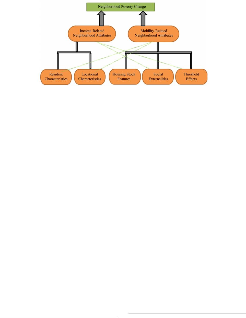 C. H. REN, H. MORROW-JONES OPEN ACCESS Figure 1. The conceptual framework. Therefore, some variables available only in certain census years are not included. Since our study only focuses on the 1990- 2000 Period and use variables that were defined consistently in both of these two census years, we do not expect to see signifi- cant biases and inaccuracies. REIS is the acronym for the Regional Economic Information System created by the Bureau of Economic Analysis (BEA) to make available employment information by detailed industrial file and at different geographic levels. In this study, all the em- ployment-related variables are calculated based on REIS.1 Study Areas This study is based in the 100 largest metropolitan areas at the time of the 1990 census as measured by the size of popula- tion. A metropolitan area typically has one or several popula- tion centers surrounded by suburban counties. The Census Bu- reau defines several types of metropolitan areas. There are stand-alone Metropolitan Statistical Areas, known as standard MSAs, Consolidated Metropolitan Statistical Areas (CMSAs) and Primary Metropolitan Statistical Areas (PMSAs). PMSAs are component units of CMSAs. The metropolitan areas defined in this study include both MSAs and PMSAs. CMSAs are ex- cluded because they are too large to be representative of unified housing and labor markets (Jargowsky, 2003), and therefore can not ensure competitive relationship between component neighborhoods. Appendix A shows a list of the 100 largest MSAs and PMSAs by population size. Unit of Analysis Consistent with previous work (Fogarty, 1977; Galster & Mincy, 1993; Galster et al., 2003; Kingsley & Pettit, 2003; Jar- gowsky, 2003; Rosenthal, 2007; Ellen & O’Regan, 2007), cen- sus tracts are used as proxies for urban neighborhoods. “census tracts are usually delineated by bounding features such as roads or rivers, and are supposed to have relatively homogeneous attributes with regard to economic, social and housing stock characteristics” (Jargowsky, 2003). Some urban scientists sug- gest that using block groups might be a better choice (Schuler et al., 1992). However many important socioeconomic variables are not available at the block group level. Also, using census tracts is consistent with most of the previous studies, making it easier to conduct historical comparison (Ellen, 2000). Therefore, although not perfect, census tracts are the best approximations to neighborhoods available for the quantitative analysis. The terms “neighborhood” and “census tract” are used interchange- ably in the remainder of this paper. The Dependent Variable The poverty rate is defined by the US Census Bureau as a percentage of the residents living below the Census Bureau Poverty Line. That is, a person is considered poor if he or she lives in a family with an income less than the Census Bureau Poverty Standard which is meant to reflect the costs of buying life necessities in the area and adjusted for inflation and family size (Jargowsky, 2003). There has been no academic consensus on what poverty rate cutoffs should be used to classify neighborhood into different categories. Scholars use varying cut off values, depending on specific emphases of the research. Jargowsky and Bane (1990), Kasarda (1993) and Jargowsky (1997), for example, used a 40% poverty rate as the threshold to distinguish “ghettos” from mixed-income neighborhoods and this cutoff is chosen primar- ily based on the experienced researchers’ observations of phys- ical appearance in the neighborhoods. Galster and colleagues (2003) used the 20% poverty rate as the cut off between mod- erate-poverty and high-poverty neighborhoods and the 40% poverty as the cut off between high-poverty and extremely high-poverty neighborhoods. Those cut off values are chosen because historical studies indicate exacerbated social problems once poverty rates exceed such threshold values (Galster et al., 2003). In this study, we employ 10% and 20% poverty rates as the cutoff values to distinguish moderate-poverty neighborhoods from low-poverty and high-poverty neighborhoods2. If a census tract has between 10% and 20% residents living below the Census Bureau Poverty Level, it’s classified as a moderate- There is an inconsistency with regard to MSA boundaries between R EIS and NCDB. To deal with this problem, REIS MSAs are broken down into counties and reorganized to match the boundaries of NCDB. Low-poverty, high-poverty and extremely high- poverty n eighborhoods are defined as those with below 10% poverty rates, between 20% and 40% poverty rates, and above 40% poverty rates. Refer to appendix table B for descriptive statistics of these different poverty-level tracts. C. H. REN, H. MORROW-JONES OPEN ACCESS poverty neighborhood. The dependent variable in this study is defined as the absolute difference in neighborhood poverty rate between 1990 and 2000. Explanatory Variables As discussed in the conceptual framework, this research in- tends to use a neighborhood’s relative competitive position in the metropolitan area to explain the variation in future poverty rate change. Most prior work calculates a neighborhood’s rela- tive position in terms of a certain attribute by using a ratio of the value of the neighborhood to the average value of the MSA (Rosenthal, 2007; Ellen & O’Regan, 2007). In this study, how- ever, the measure of a neighborhood’s position relative to the entire MSA holds less explanatory power, because neighbor- hoods in different economic status categories usually do not have a direct competitive relationship. Therefore, in this study, a neighborhood’s relative competitive status in terms of a cer- tain attribute is measured by using a ratio of the neighborhood value to the average value of all neighborhoods of the same poverty category in the MSA. For example, a moderate-poverty neighborhood’s relative competitive position measured by ho- meownership rate is calculated by a ratio of the neighborhood homeownership rate to the average homeownership rate of all moderate-poverty neighborhoods in the MSA. All neighbor- hood-level variables used in this study are measured this way except for dummy variables. The purpose of this measurement is to ensure that neighborhoods within a metropolitan area form a direct competitive relationship with each other, which is the fundamental idea of this study. Based on the conceptual framework and past empirical stu- dies, a set of explanatory variables are selected to measure a neighborhood’s relative competitive position within the MSA (See Table 1 for the detailed descriptions of the variables, and table B in the Appendix section for their descriptive statistics). In the model, the dependent variable is measured by decadal changes 1990-2000, and most explanatory variables are in be- ginning-of-period values while some of them are changes in the previous decade. The idea is that the beginning-of-period val- ues of a neighborhood’s attributes are predictive of its future course of poverty transition in the next decade. Dummy va- riables are added to test possible threshold effects of the se- lected neighborhood attributes. Discussion of Model Results Originally there are 17,986 NCBD census tracts that have a moderate poverty status. After excluding 10,172 inappropriate tracts, the reported results are based on 7814 moderate poverty census tracts in the 100 largest US metropolitan statistical areas. The excluded tracts include 1) those not located in the 100 largest MSAs (in rural areas or small MSAs); 2) those with 0 population or 0 poverty-status determined population in 1980 and 2000; 3) those with a population less than 100 in 1990; 4) those with 0 families in 1990; 5) those with 10% or more of their populations in mental hospital or juvenile institutions; 6) those with 40% or more of their populations in military institu- tions, college dormitories, other institutions and non-institu- tional quarters. Overview Table 2 shows model results based on the Ordinary Least Square regression (OLS). The R-squared statistic is 0.202, which is a typically low value for models predicting neighbor- hood poverty change. Almost all the estimated coefficients are significant with the expected signs. This is very rare compared with previous studies, indicating that using a neighborhood’s relative competitive position to predict its future course of po- verty transition generally works well. Income-Related Neighborhood Attributes Consistent with historical findings (Scott, 1988; Galster & Mincy, 1993), low educational attainment in a neighborhood is found to be a negative characteristic that puts the neighbor- hood’s residents in an unfavorable position in employment markets. One possible explanation for the positive coefficient on Foreign90 is that new immigrants still suffer from a lan- guage barrier and the lack of middle-class social connection. Although some prior studies suggest that there might be posi- tive effects due to their support network based on homogeneous backgrounds, such effects are found to be minor in moderately poor areas. A relatively higher proportion of female-headed families also makes the neighborhood more likely to experience poverty growth. It is not possible to tell with the available data if this affects poverty rate change through welfare dependency or by giving women additional difficulty in job market compe- tition or in some other manner. The variable NoCar90 is used to test the effect of automobile ownership on people’s competi- tive position in employment markets. As it turns out, in mod- erate-poverty neighborhoods, the relative lack of transportation means significantly limits people’s access to job opportunities (Galster & Mincy, 1993). Finally, a neighborhood that has a relatively larger portion of married-couple familie s i s less li kely go through poverty growth, which indic ates marriage ’s positive role in resisting economic hardship, be it financially or psycho- logically. Two variables are included to test a neighborhood’s loca- tional disadvantages or advantages in its residents’ access to employment opportunities. Both Access-To-Local-Job90 and Distance-To-CBD90 turn out to be significant, but the influ- ence of the distance to CBD is much greater than the proximity to local jobs. This indicates that in an age of advanced trans- portation technologies, whether or not a neighborhood is lo- cated in a job-rich community is no longer a crucial factor in determining its residents’ access to job opportunities, and people depend more on more distant metropolitan employment opportunities than local ones. Those findings are also consistent with the significant positive coefficient on NoCar90, which implies the importance of automobile ownership. Mobility-Related Neighborhood Attributes As discussed earlier, when it comes to the effect of old housing stock on neighborhood poverty status change, con- flicting evidence is present in the urban literature. The results from this research indicate that a moderate-poverty neighbor- hood is expected to experience less poverty growth if it has a larger proportion of old housing units or a larger proportion of new housing units. So evidence is found to support Ellen and O’Regan (2007) and Rosenthal’s (2007) proposal that as a neighborhood becomes older, its chance of receiving major reinvestment increases, which will elevate its economic status in the next decade. The coefficient of the variable vacancy90  C. H. REN, H. MORROW-JONES OPEN ACCESS Table 1 . The de s crip tio ns of t he v a riab le s. Expected Sign Resident Characteristic s Proportion of Residents Aged 25+ Who Complete 0 - 8 Years of School i n Tract in 1990/The Counterpart in + -Born Resi dents in Tract in 1990/The Counterpart in MSA in 1990 + -Couple Familie s in Tract in 1990/The Counterpart in MSA in 1990 − -Headed90 -Headed Families in Tract in 1990/The Counterpart in MSA in 1990 + Proportion of Househol ds Without a C ar in Tract i n 1990/The C ount erpart in MSA in 1990 + Characteristics -To-Local-Job90 -Population Ratio in County in 199 0/The Counterpart in MSA in 1990 − -To-CBD90 The Tract’ s Distance to CBD in 1990/T he Counterpart in MSA in 19 90 + Housing Stock Ch arac te ri st ic s Proportion of Housing Units Aged 50+ in Tract in 1990/The C ount erpart in MSA in 1990 − Proportion of Housing Units Aged 5 − in Tract in 1990/The Counterpart in MSA in 1990 − Housing Vacancy Rate i n Tract in 1990/The Counterpart in MSA in 1990 + Tract Pove rt y Rate in 1990/The Counte rpart in MSA in 1990 − -90 (Tract Pove r t y Rate in 1990/The Count erpart in MSA in 1990) - (Tract Poverty Rate in 1980/The Counterpart − -To-20Pov90 The Tract’ s Distance to t he Neare st Tract with 20%+ Poverty Rate in 1990/The Counterpart in MSA in 19 90 + -To-40Pov90 The Tract’ s Distance to t he Neare st Tract with 40%+ Poverty Rate in 1990/The Counterpart in MSA in 1990 + -American Residents in Tract in 1990/The C ount erpart in MSA in 1990 + -90 -American Residents in Tract in 1990/The Coun t erpart in MSA in 1990) (Proportion of African-American Residents in Tract in 1980/The Counter part in MSA in 1980) + Proportion of Hispanic Residents in Tract in 1990/The Count erpart in MSA i n 1990 + -Density90 Tract Population Density in 1990/T he Counterpart in MSA i n 1990 + with an Annual Income $60000+ in Tract in 1990/T he Counterpart in MSA in 1990 − Proportion of Residents Aged 16+ in Executives, Managers or Administrators in Tract in 1990/The Counte r part − Tract in 1990/The Counterpart in MSA in 1990 − Proportion of Residents Aged 25+ with a College Degree/The Counterpart in MSA in 1990 − Proportion of Househol ds Who Have R es i ded in the Tract for More T han 5 Years/The Counterpart in MSA − a Proportion of Families with Own Chil dren in Tract in 1990/The Counterpa rt in MSA in 19 90 -Dummy-1 The Variable Poverty90 Exceeds One Standard Deviation Above Its Mean − -Dummy-2 The Variable Poverty90 Exceeds Two Standard Deviation Above Its Me an − -Dummy-1 The Variable Black90 Exceeds One Standard Deviation Above Its Mean + -Dummy-2 The Variable Black90 Exceeds Two Standard Deviation Above Its Me an + Note: aFamilies with of children are known to be more sensitive to the neighborhood environment, and therefore are expected to have a relatively higher likelihood of moving out if there’s a sign of decline. So the variable “Propwithchild90” is created to control for this effect. exhibits a significantly positive coefficient. So the expected negative effect of vacant housing units is confirmed. In mod- erate-poverty areas, neighborhoods with higher housing vacan- cy rates appear less appealing to relatively affluent households and those neighborhoods are more likely to slip into concen- trated poverty. When it comes to social externality effects, Pop-Density90 proves to have a positive impact on poverty rate increase. So neighborhoods with relatively higher population density are in a disadvantaged position in the competition for more affluent  C. H. REN, H. MORROW-JONES OPEN ACCESS Table 2. Results of moderate poverty tracts. (Adjusted R-squared = 0.202; N = 7814) Explanatory Variables Coefficient Std-Erro r T-value Constant 0.0179 0.0144 1.2444 Resident Characteristics Lowedu90 0.0699*** 0.0154 4.5498 Foreign90 0.0951*** 0.0130 7.3233 Married90 −0.0628*** 0.0197 −3.1898 Female-Headed90 0.0728*** 0.0211 3.4515 Nocar90 0.1092*** 0.0144 7.5605 Place Characteristics Access-To-Local-Job90 −0.0385*** 0.0113 −3.4109 Distance-To-CBD90 0.0661*** 0.0189 3.5041 Housing Stock Charac te ri stic s ProOldHou90 −0.0465*** 0.0117 −3.9688 ProNewHou90 −0.0559*** 0.0119 −4.6846 Vacancy90 0.0644*** 0.0114 5.6677 Social Externalitie s Poverty90 −0.2262*** 0.0172 −13.1856 Poverty80-90 −0.0749*** 0.0116 −6.4587 Distance-To-20Pov90 −0.0897*** 0.0155 −5.7894 Distance-To-40Pov90 −0.0898*** 0.0201 −4.4730 Black90 0.1376*** 0.0218 6.3235 Black80-90 0.0693*** 0.0112 6.1720 Hispanic90 −0.0083 0.0122 −0.6797 Pop-Density90 0.0748*** 0.0107 6.9659 HighIncome90 −0.031* 0.0168 −1.8439 Highpro90 −0.0697*** 0.0153 −4.5482 Homeowner90 −0.0969*** 0.0168 −5.7823 Highedu90 −0.1071*** 0.0212 −5.0617 Move5years90 −0.0515*** 0.0168 −3.0657 The Control V ariable Propwithchild90 0.0114 0.0150 0.7599 Dummy Var i abl es Poverty90-Dummy-1 −0.0132 0.039 −0.3383 Poverty90-Dummy-2 −0.1257 0.0774 −1.6251 Black90-Dummy-1 −0.0439 0.054 −0.8133 Black90-Dummy-2 −0.166** 0.0732 −2.2698 Note: Al l estimates are produced by SP SS 13, using standardized sc ores. *P < 0.1, **P < 0.05, ***P < 0.01. residents. Following Rosenthal’s approach (2007), we use den- sity as an indirect measure for the level of criminal activities. Density can also serve as a proxy for many other poverty- related factors. For example, while higher-density neighbor- hoods are expected to frighten away wealthier famili es because of their perceived higher crime rates, it is also plausible that people might be actually deterred by the higher tax rates, and poorer quality schools of central city communities since higher- density neighborhoods are more likely to be located in central city areas. With limited data sources, it is not possible to diffe- rentiate between these possible poverty-generating mechan- isms. On the social capital side, all four variables exhibit signifi- cantly negative coefficients as expected. Neighborhoods with C. H. REN, H. MORROW-JONES OPEN ACCESS relatively higher proportions of high-income families, college graduates and residents with high-status jobs, have an advan- taged competitive position in the metropolitan area, and there- fore are likely to experience less poverty growth. The social capital created by these variables makes a neighborhood more appealing and works as an attractor for affluent families. On the other hand, they are also supposed to help the incumbent neighborhood residents thrive by providing positive role mod- els and increasing social interaction in the community (Rosen- thal, 2007; Ellen & O’Regan, 2007). As the most prominent social capital generator as proved by numerous past studies (Brueckner, 1977; Carter et al., 1998; Galster et al., 2003; Ellen & O’Regan, 2007; Rosenthal, 2007), homeownership’s role in resisting poverty growth is confirmed in this study. The varia- ble Move5Years90 represents the proportion of the households who have resided in the neighborhood for more than 5 years. The significantly negative sign of this variable supports the view that neighborhood stability helps to resist future poverty growth. The analysis results report a positive correlation between the relative proportion of African Americans and future neighbor- hood poverty growth. The past racial transition trend (Black80- 90) proves to be influential as well. Those findings indicate that relatively high percentages of African-American residents are still associated with declines in moderate-poverty urban areas where there is often a relatively large white population. The findings provide support for Ellen’s (2000) “race-based neigh- borhood stereotyping hypothesis” that although pure racial prejudice has lost its popularity, white people still tend to use race as a measure to estimate future neighborhood quality when making residential location decisions. The model results also show that once the relative proportion of African-American residents exceeds two standard deviations above the mean, the negative effect of Black90 is significantly muted. This result confirms the other side of racial effects. That is, once the percentage of minority residents surpasses certain thresholds the large share of minorities becomes a neighbor- hood stabilizer. This supports the idea that African Americans can take advantage of race-based support networks to cope with economic hardship (Galster & Mincy, 1993). The relative pro- portion of Hispanic residents is irrelevant to future poverty growth in moderate-poverty neighborhoods. Four variables are created to examine the endogenous effects of concentrated poverty. Similar to racial variables, Poverty90 and Poverty80-90 are used to test the effects of income tipping and the past trend of income transition. Distance-To-20Pov90 and Distance-To-40Pov90 are used to evaluate the spill-over or border effects of concentrated poverty. Some interesting results are found. Consistent with conven- tional wisdom, the two distance variables have negative coeffi- cients which mean that proximity to concentrated poverty con- tributes to future poverty increase. However, the signs for the coefficients of both Poverty90 and Poverty80-90 are signifi- cantly negative. These results suggest that a neighborhood will go through more poverty growth if it is located closer to other neighborhoods with high poverty rates, but it will experience less poverty growth if it has a relatively higher poverty status itself. It seems unreasonable that affluent households would be at- tracted to neighborhoods with relatively higher poverty status, while in the meantime trying to avoid those with proximity to concentrated poverty. One explanation is that strong policy intervention has been involved in the neighborhood poverty transition process during the 1990s. As Ellen and O’Regan (2007) suggest, numerous anti-poverty initiatives were put into practice during this period. These include strict enforcement of anti-discrimination laws in housing markets, welfare reforms, and other programs designed to promote employment rates among the working poor. With those anti-poverty efforts, the presence of a higher proportion of poor individuals actually increases a neighborhood’s chance of receiving government assistance and therefore makes it less likely to experience po- verty growth in the subsequent decade. The two distance va- riables mainly reflect the effects of natural economic forces. In summary, our quantitative model works well to explain the course of poverty transition of moderate-poverty neighbor- hoods in US metropolitan areas. In general, neighborhoods with attributes that gives them advantages in the inter-neighborhood competition, show better ability to resist future poverty increase. These attributes include a relatively larger proportion of mar- ried couple families, a relatively larger proportion of home- owners, and so on. On the other hand, neighborhoods with at- tributes that gives them disadvantages in the inter-neighborhood competition, are more subject to future poverty growth. These attributes include a relatively higher density, relatively larger African American population and so on. Conclusions, Discussion and F uture Research Directions Conclusions and Policy Implications Concentrated poverty has long been a focus in the urban lite- rature, but most of the previous studies focus on areas that al- ready have high concentrations of poverty in the hope of help- ing these distressed urban areas get out of impoverished condi- tions. This study is intended to complement the urban poverty literature by discovering poverty dynamics patterns in mod- erately poor urban areas, so that policies can be made to inter- vene in the process by which poverty gets concentrated. A competitive model is established to explore the course of neigh- borhood poverty concentration. Several important findings are revealed and they lead to interesting policy recommendations. Most of anti-poverty programs are reactive rather than pre- ventive in nature. That is, they tend to target already poor urban neighborhoods in the hope of poverty deconcentration instead of working on moderately poor areas to impede the downward filtering process. Some urban programs apply a place-oriented approach, such as the empowerment zone (EZ) which offers tax breaks and other policy benefits to attract business investments to upgrade distressed areas. Some programs rely on a people- oriented perspective and aim to fight concentrated poverty by helping poor individuals directly, such as community training programs and the moving to opportunity (MTO) program (Temkin & Rohe, 1996). All these programs underplayed the fact that the best way to fight concentrated poverty is to prevent poverty from getting concentrated. The policy emphasis, there- fore, should be shifted towards these areas where noticeable amount of poverty is present but the magnitude is not signifi- cant enough to cause substantial socials problems and subse- quent income tipping. The important finding of the competitive model applied in this study is that neighborhood poverty status is a dynamic process instead of a static phenomenon. As a result of intensive inter-neighborhood competitions, those with unfavorable posi-  C. H. REN, H. MORROW-JONES OPEN ACCESS tions will keep declining, eventually leading to concentrated poverty and a stratified metropolis pattern. Also, when it c omes to poverty rate transition due to people’s mobility patterns, some neighborhoods’ gains of affluent households are others’ losses. From a local perspective, some communities may be- come the winners of the competition and experience growth in economic status, but for the region as a whole, it is a zero-sum game at best (Orfield, 2002). Therefore, to prevent the stratifi- cation of metropolitan patterns and wasteful competition, a regional perspective is needed when enacting and implementing public policies, and some type of governing body at the metro- politan level is required to coordinate local efforts. The findings of this research also provide a rich set of em- pirical results needed for enacting specific policies. For exam- ple, those areas with a large body of residents in disadvantaged competitive positions should be given more attention by policy makers, such as neighborhoods with a higher percentage of female-headed families or a higher percentage of new immi- grants. Automobile ownership is another significant factor in explaining neighborhood poverty growth, indicating the impor- tance of transportation means for gaining access to job oppor- tunities. A well-developed public transit system might fill this vacancy and therefore increase an area’s ability to resist pover- ty growth. Evidence to support central-city revitalization programs is found in this study also. Although decentralization has become the dominant pattern of economic activities, people living in moderately poor urban areas still have heavy reliance on CBD jobs. This finding also conforms to what observed by Downs (1994) who contends that central cities are still desirable loca- tions for a wide variety of industries. Future Research Directions This study contributes to the urban poverty literature by ex- ploring the poverty succession mechanisms in moderate-po- verty neighborhoods. From a practical perspective, a set of poverty change predictors are identified, which can serve as the basis for formulating anti-poverty policies targeting particularly moderately poor neighborhoods to prevent them from degrad- ing into high-poverty areas. From a theoretical perspective, this study enriches the existing urban poverty literature with its model of explaining neighborhood poverty dynamics through the inter-neighborhood competition. It should be noted that this study is an initial step in model- ing neighborhood poverty change from an inter-neighborhood- competition perspective. There are several important limitations that we hope can be overcome by future research. To begin with, a richer set of explanatory variables might help to improve the model. For example, many possible poverty- change indicators are not available in NCDB and REIS, the two major datasets used in this study. We have no direct measure for school quality which is probably the most important factor to consider when a family makes residential choices. Also, the explanatory power of the model might be significantly ex- panded if influential factors at larger geographical scale could be added, such as metropolitan demographic change s and larger- scale econom i c dynamics. In addition, we carefully selected explanatory variables in order to separate the effects of the two poverty-generating me- chanisms: incumbent income changes and selective migration. The results were unexpected in that most neighborhood-level variables affect poverty transition through both of the two processes. For example, a higher proportion of college gra- duates generates higher levels of social capital and therefore elevates the economic status of the neighborhood by attracting more affluent families. On the other hand, these highly-edu- cated people themselves are in a favorable position in employ- ment markets and can also help the rest of the neighborhood residents prosper through positive role-model effects. A single city or single metro case study with more detailed information will work better to distinguish between the effects of these two mechanisms. Finally, we relied solely on the traditional OLS method to perform statistical analyses. The accuracy of the results will certainly be improved if more sophisticated statistical ap- proaches can be employed, such as using spatial regression models to take care of spatial autocorrelation and applying simultaneous equation modeling to explore complex interac- tions of different neighborhood attributes. The primary purpose of this study is to provide a new framework for understanding the dynamics of moderately poor urban areas and to perform a first test of its usefulness. As more elements are added by future research, especially with the newly-released Census 2010 data, we hope the model proposed in this study will give us a deeper insight into the neighborhood transition mechanisms. REFERENCES Brueckner, J. (1977). The determinants of residential s uccession. Jour- nal of Urban Econ omics, 4, 45-59. http://dx.doi.org/10.1016/0094-1190(77)90029-8 Carter, W. H., Schill, M. H., & Wachter, S. M. (1998). Polarisation, public housing and racial minorities in US cities. Urban Studies, 35, 1889-1911. http://dx.doi.org/10.1080/0042098984204 Cohen, C. J., & Dawson, M. C. (1993). Neighborhood poverty and African American politics. American Political Science Review, 87, 286-302. http://dx.doi.org/10.2307/2939041 DiPasquale, D., & Glaeser, E. L. (1999). Incentives and social capital: Are homeowners better citizens? Journal of Urban Economics, 45, 354-384. http://dx.doi.org/10.1006/juec.1998.2098 Downs, A. (1994). New vision for metropolis America: Why we need a new vision. Washington, DC: Brookings Institution. Eggers, M. L., & Massey, D. S. (1992). A longitudinal analysis of urban poverty: Blacks in U.S. metropolitan areas between 1970 and 1980. Social Science Research, 21, 175-203. http://dx.doi.org/10.1016/0049-089X(92)90014-8 Ellen, I. G. (2000). Sharing America’s neighborhoods: The prospects for stable, racial integration. Cambridge, MA: Harvard University Press. Ellen, I. G., & O’Regan, K. (2007). Reversal of fortunes? Lower- income urban neighborhoods in the US in the 1990s. Urban Studies, 45, 845-869. Fogarty, M. S. (1977). Predicting neighborhood decline within a large central city: An application of discriminant analysis. Environment and Planning A, 9, 579-584. http://dx.doi.org/10.1068/a090579 Galster, G. C. (2001). On the nature of neighborhood. Urban Studies, 38, 2111-2124. http://dx.doi.org/10.1080/00420980120087072 Galster, G. C., Quercia, R. G., Cortes, A., & Malega, R. (2003). The Fortunes of poor neighborhoods. Urban Affairs Review, 39, 205-227. http://dx.doi.org/10.1177/1078087403254493 Hughes, M. (1989). Mispeaking truth to power: A geographical pers- pective on the “underclass” fallacy. Economic Geography, 65, 187- 207. http://dx.doi.org/10.2307/143834 Jargowsky, P. (1997). Poverty and place: Ghettos, barrios, and the American city. New York: Russell Sage Foundation. Jargowsky, P. (2003). Stunning progress, hidden problems: The dra-  C. H. REN, H. MORROW-JONES OPEN ACCESS matic decline of co ncentra ted pover ty in the 1990s. Washington, DC: Brookings Institution Press. Jargowsky, P., & Bane, M. J. (1990). GHETTO poverty: Basic ques- tions. In Inner-city poverty in the United States. Washington, DC: National Academy Press. Kasarda, J. (1993). Inner-city concentrated poverty and neighborhood distress: 1970 to 1990. Housing Policy Debate, 4, 253-302. http://dx.doi.org/10.1080/10511482.1993.9521135 Kingsley, G. T., & Pettit, K. (2 00 3). Co ncen tra ted po verty: A change in course. Washington, DC: The Urban Institute. Leven, C., Little, J., Nourse, H., & Read, R. (1976). Neighborhood change: Lessons in the dynamics of urban decay. New York: Pr aeger Publishers. Massey, D. S., & Eggers, M. L. (1990). The ecology of inequality: Minorities and the concentration of poverty, 1970-1980. American Journal of Sociology, 95, 1153-1188. http://dx.doi.org/10.1086/229425 Massey, D., Eggers, M., & Denton, N. (1990). Disentangling the causes of concentra ted poverty. Unpublished Paper, Chicago, IL: Population Research Center, NORC/University of Chicago. Metzger, J. (2000). Planned abandonment: The neighborhood life-cycle theory and national urban policy. Housing Policy Debate, 11, 7-40. http://dx.doi.org/10.1080/10511482.2000.9521359 Mincy, R. B., Sawhill, I., & Wolf, D. (1990). The underclass: Defini- tion and measurement. Science, 248, 450-453. http://dx.doi.org/10.1126/science.248.4954.450 Oreopoulos, P. (2003). The long-run consequences of growing up in a poor neighborhood. Quarterly Journal of Economics, 118, 1533- 1575. http://dx.doi.org/10.1162/003355303322552865 Orfield, M., & Katz, B. (2002). American metropolitics: The new sub- urban reality. Washington, DC: Brookings Institution Press. Quercia, R. G., & Galster, G. C. (20 00). Thresh-old effects and neigh- borhood change, Journal of Planning Education and Research, 20, 146-162. http://dx.doi.org/10.1177/0739456X0002000202 Rosenthal, S. (2007). Old homes, externalities, and poor neighborhoods: A model of urban d ecline and ren ewal. Journal of Urban Economics, 63, 816-840. http://dx.doi.org/10.1016/j.jue.2007.06.003 Schuler, J., Kent, R., & Monroe, B. (1992). Neighborhood gentrifica- tion: A discriminant analysis of a historic district in Clev eland, Ohio. Urban Geography, 13, 49-67. http://dx.doi.org/10.2747/0272-3638.13.1.49 Scott, A. (1988). Metropolis: From division of labor to urban form. Berkeley, CA: University of California Press. Tatian, A. P. (2003). Neighborhood change database: Data users’ guide. http://www.geolytics.com/pdf/NCDB-LF-Data-Users-Guide.pdf Temk in , K., & Robe, W. (1996). Neighborhood change and urban policy. Journal of Planning Education and Research, 15, 159-170. http://dx.doi.org/10.1177/0739456X9601500301 Wilson, W. J. (1987). The truly disadvantaged. Chicago, IL: The Uni- versity of Chicago Press.  C. H. REN, H. MORROW-JONES OPEN ACCESS Appendix Table A. The 100 largest MSAs. Rank MSA Na me Population (1990) Population (2000) 1 Los Angeles-Long Beach-Santa Ana, CA 8,803,804 9,463,883 2 New York-Northern New Jersey-Long Island, NY-NJ-PA 8,485,881 9,261,473 3 Chicago-Joliet-Naperville, IL-IN-WI 7,263,100 8,107,644 4 Philadelphia-Camden-Wilmington, PA-NJ-DE-MD 4,853,879 5,037,277 5 Detroit-Warren-Livonia, MI 4,256,681 4,429,015 6 Washington-Arlington-Alexandria, DC-VA-MD-WV 3,915,023 4,537,017 7 Houston-Sugar Land-Baytown, TX 3,317,651 4,162,976 8 Boston-Cambridge-Quincy, MA-NH 3,163,429 3,349,729 9 Atlanta-Sandy Springs-Marietta, GA 2,659,377 3,712,871 10 Nassau-Suffolk, NY PMSA 2,588,748 2,740,474 11 Riverside-San Bernardino-Ontario, CA 2,553,696 3,216,638 12 Dallas-Fort Worth-Arlington, TX 2,539,540 3,312,284 13 Minneapolis-St. Paul-Bloomington, MN-WI 2,470,395 2,888,515 14 St. Louis , MO-IL 2,465,930 2,575,551 15 San Die go-Carlsbad-San Marcos, CA 2,411,260 2,682,438 16 Orange County, CA PM SA 2,406,318 2,772,046 17 Baltimore-Towson, MD 2,317,207 2,478,515 18 Pittsburgh, PA 2,229,272 2,190,442 19 Phoenix-Mesa-Glendale, AZ 2,224,932 3,114,937 20 Cleveland-Elyria-Mentor, OH 2,190,554 2,235,084 21 San Francisco-Oakland-Fremont, CA 2,061,150 2,377,318 22 Seattle-Tacoma-Bellevue, WA 1,967,708 2,340,497 23 Tampa-St. Petersburg-Clearwater, FL 1,963,580 2,248,952 24 Miami -Fort Lauderdale-Pompano Beach, FL 1,932,629 2,228,236 25 Newark, NJ PMSA 1,892,972 2,009,948 26 Denver-Aurora-Broomfield, CO 1,614,261 2,073,249 27 San Francisco-Oakland-Fremont, CA 1,601,830 1,729,392 28 Kansas City, MO-KS 1,509,671 1,689,903 29 San Jose-Sunnyvale-Santa Clara, CA 1,486,159 1,670,333 30 Portland-Vancouver-Hillsboro, OR-WA 1,477,750 1,874,313 31 Cincinnati-Middletown, OH-KY-IN 1,449,682 1,555,636 32 Milwaukee-Waukesha-West Allis, WI 1,424,494 1,493,311 33 Virginia Beach-Norfolk-Newport News, VA-NC 1,376,102 1,521,625 34 Indianapolis-Carmel, IN 1,374,677 1,603,105 35 Fort Wort h-Arlington, TX PMSA 1,353,764 1,691,352 36 Columbus, OH 1,334,674 1,523,881 37 Sacramento-Arden-Arcade-Roseville, CA 1,333,407 1,540,760 38 San Anto nio-New Braunfels, TX 1,287,621 1,541,284 39 Bergen-Passaic, NJ PMSA 1,277,980 1,372,791 40 Fort La uderdale-Hollywood-Pompano Beach, FL PMSA 1,255,242 1,530,737 41 New Orleans-Metairie-Kenner, LA 1,214,326 1,266,582 42 Orlando-Kissimmee-Sanford, FL 1,213,005 1,632,377 43 Buffalo-Niagara Falls, NY 1,178,011 1,161,926 44 Hartford-West Hartford-E ast Ha rtfo rd, C T 1,133,991 1,167,171 45 Providence-New Bedford-Fall River, RI-MA 1,116,411 1,170,823 46 Charlotte-Gastonia-Rock Hill, NC-SC 1,109,365 1,433,620  C. H. REN, H. MORROW-JONES OPEN ACCESS Continued 47 Salt Lake City, UT 1,070,600 1,326,965 48 Greensboro-High Point, NC 1,006,213 1,200,117 49 Middlesex-Somerset-Hunterdon, NJ PMSA 985,716 1,139,643 50 Rochester, NY 985,477 1,023,027 51 Memphis, TN-MS-AR 985,090 1,122,347 52 Monmouth-Ocean, NJ PMSA 983,890 1,125,219 53 Nashville-Davidson-Murfreesboro-Franklin, TN 971,835 1,218,485 54 Dayton, OH 947,571 946,566 55 Grand Rapids-Wyoming, MI 937,836 1,088,426 56 Oklahoma City, OK 922,673 1,040,958 57 Louisville-Jefferson County, KY-IN 895,404 966,034 58 Jacksonville, FL 894,351 1,094,171 59 West Palm Beach, FL SM SA 860,943 1,127,640 60 Richmond, VA 850,439 978,327 61 Birmingham-Hoover, AL 840,139 921,106 62 Honolul u, HI 818,435 831,910 63 Albany-Schenectady-Troy, NY 812,897 828,822 64 Raleigh-Cary, NC 790,272 1,110,405 65 Greenville-Mauldin-Easley, SC 774,278 899,596 66 Austin-Round Rock-San Marcos, TX 763,024 1,142,566 67 Fresno, CA 754,474 917,162 68 Las Vegas-Paradise, NV 740,120 1,121,269 69 Tulsa, OK 704,606 796,096 70 Oxnard-Thousand Oaks-Ventura, CA 661,917 746,186 71 Tucson, AZ 658,178 832,275 72 Syracuse, NY 637,106 631,198 73 Akron, OH 633,030 670,905 74 Omaha-Council Bluffs, NE-IA 614,525 672,601 75 Toledo, OH 603,579 608,454 76 Gary, IN PMSA 599,556 626,703 77 Allentown-Bethlehem-Easton, PA-NJ 592,210 636,936 78 El Paso, TX 591,248 673,263 79 Harrisburg-Carlisle, PA 587,987 629,401 80 Seattle-Tacoma-Bellevue, WA 579,782 693,485 81 Springfield, MA 568,257 571,903 82 Jersey City, NJ SMSA 552,992 608,811 83 Scranton-W ilkes-Barre, PA 547,267 532,545 84 Albuquerque, NM 541,723 637,528 85 Bakersfield-Delano, CA 537,646 644,418 86 New Haven-Milford, CT 524,742 535,921 87 Baton Rouge, LA 517,085 590,591 88 Wilmington, NC 508,170 579,329 89 Knoxvil l e, TN 496,577 569,133 90 Charle st on, WV 494,596 543,387 91 Youngstown-Warren-Boardman, OH-PA 492,699 482,671 92 North Port-Bradenton-Sarasota, FL 489,487 583,940 93 Wichita, KS 485,269 545,220 94 Stockton, CA 473,856 547,774 95 Worcester, MA 471,667 504,396 96 Mobile, AL 469,485 533,071  C. H. REN, H. MORROW-JONES OPEN ACCESS Continued 97 Little Rock-Nort h Little Rock-Conway, AR 451,305 496,830 98 Bridgeport-Stamford-Norwalk, CT 441,589 457,968 99 Vallejo-Fairfield, CA 434,757 511,287 100 Johnson City, TN 433,915 478,035 Source: The Burea u of Economic Analysis’ Re gional Informati on System (REIS). Table B. Descriptive statistics for different poverty-level tracts. Dependent Variable Mod-Poverty Tracts High-Poverty Tracts Ex-Poverty Tracts N Mean STD N Mean STD N Mean STD Povratechange90-00 7814 0.0106 0.0599 5221 −0.0064 0.0797 1946 −0.0896 0.1133 Resident Characteristic s Lowedu90 7814 0.1182 0.0758 5221 0.1973 0.1167 1946 0.2270 0.1152 Foreign90 7814 0.1320 0.1515 5221 0.1695 0.1901 1946 0.1008 0.1445 Married90 7814 0.7322 0.1003 5221 0.5858 0.1385 1946 0.3905 0.1708 Female-Headed90 7814 0.1365 0.0651 5221 0.2355 0.1023 1946 0.3892 0.1494 Nocar90 7814 0.1562 0.1422 5221 0.2987 0.1866 1946 0.5258 0.2056 Place Characteristics Access-To-Local-Job90 7814 0.9890 0.3088 5221 1.0519 0.3717 1946 1.0667 0.4330 Distance-To-CBD90 7814 14.7510 14.2428 5221 10.1450 12.4403 1946 6.0768 7.6611 Housing Stock Ch arac te ri st ic s ProOldHou90 7814 0.2314 0.2527 5221 0.3150 0.2553 1946 0.3457 0.2270 ProNewHou90 7814 0.0821 0.1035 5221 0.0546 0.0778 1946 0.0376 0.0605 Vacancy90 7814 0.0841 0.0665 5221 0.1071 0.0674 1946 0.1408 0.0954 Social Externalitie s Poverty90 7814 0.1416 0.0286 5221 0.2822 0.0567 1946 0.5119 0.1039 Poverty80-90 7814 0.0197 0.0530 5221 0.0480 0.0846 1946 0.1033 0.1112 Distance-To-20Pov90 7814 4.0659 6.7175 5221 1946 Distance-To-40Pov90 7814 10.3539 14.6089 5221 5.4683 12.3336 1946 Black90 7814 0.1578 0.2440 5221 0.3584 0.3521 1946 0.5988 0.3616 Black80-90 7814 0.0289 0.0813 5221 0.0250 0.1027 1946 0.0220 0.1210 Hispanic90 7814 0.1460 0.1911 5221 0.2438 0.2859 1946 0.2042 0.2870 Pop-Density90 7814 9406 15514 5221 14255 20921 1946 16568 23519 HighIncome90 7814 0.1506 0.0994 5221 0.0820 0.0690 1946 0.0353 0.0519 Highpro90 7814 0.1034 0.0427 5221 0.0746 0.0399 1946 0.0553 0.0390 Homeowner90 7814 0.5350 0.2128 5221 0.3974 0.2119 1946 0.2519 0.1882 Highedu90 7814 0.1666 0.1263 5221 0.1132 0.1089 1946 0.0684 0.0883 Move5years90 7814 0.4834 0.1446 5221 0.4840 0.1489 1946 0.4873 0.1468 The Control Variable Propwithchild90 7814 0.4951 0.1023 5221 0.5546 0.1052 1946 0.6118 0.1265 Note: Al l entries are based on the original dat a, as opposed to the relative measures used in t he quantitative models.
|