iBusiness, 2011, 3, 1-4
doi:10.4236/ib.2011.31001 Published Online March 2011 (http://www.SciRP.org/journal/ib)
Theoretical and P ractical Notes on Vending
Strateg ies*
Gustav Cepciansky, Ladislav Schwartz
Department of Telecommunication and Multimedia, Faculty of Electrical Engineering, University of Žilina, Zilina, Slovakia.
Received September 24th, 2010; revised November 17th, 20 10; accepted November 22nd, 2010.
ABSTRACT
The paper deals with an application of theory of mass servicing on some cases in vending strategies. The aim of the
paper is to show how the theory which is apparently applicable for scientific problems can also be utilised in practical
use. First, the necessary theoretical background will have been done and then some examples applied on vending prac-
tises will be giv e n.
Keywords: Probability, Goods, Sale, Guarantee Time, Vending Losses
1. Introduction
The theory of mass servicing is based on Markov’s ran-
dom processes. It can be applied in man y scientific areas
and technical and economical branches. For mulae of this
theory derived for stable state are well known. They are
used for calculation of service channels which can be
cash desks in department stores, seats in canteens, work
places in call centres or help desks, etc. T he results of t he
theory in stable state are widely used in telecommunica-
tion praxis at dimensioning of communication channels
and s witchi ng no des a nd als o in t heor y of reliabilit y. But
less k no wn a re the re s ult s o f t hi s t heo ry in transit io n ( no n
stable) state. Some examples can be taken from nuclear
physic, biology and radio communication. The theory in
transition state can also be applied on some economical
processes and especially on vending practises as well.
2. Theoratical Backgrond
Formula for the full probability is fundamental for our
further consid erat ion:
{ } { } {}
0
n
jj
j
PAPA .PAA
=
=∑
(1)
Here
{ }
PA
is the probability of an appearance A
that can onl y occur together with appearances
j
A
, whi c h
create the full set of mutually excluding appearances and
therefore the sum of their probabilities
{ }
j
PA
for all
12j, ,,n=
must be equal 1.
{ }
j
P AA
is the condi-
tional probability with which the appearance A occurs
together with one of the appearances
j
A
.
Let’s consider a system containing elements that grad-
ually and randomly leave the system until it gets empty.
Let denote:
n - initial number of eleme nts in the system,
τ - avera ge ti me an ele ment stays in the sys t em,
µ - nu mb er o f element s havi n g left the s yste m d ur i ng a
time uni t,
t - time,
( )
k
pt t+∆
- probability the system will contain k
elements in a f uture time
t t+∆
,
( )
j
pt
- pr obability the system co ntains j elements in a
time t,
( )
j,k
pt∆
- conditional probability the system transits
from j elements to k elements within an arbitrary short
time interval
0t∆→
.
There are only 2 possibilities how the system can get
into the state with k elements in a future time t + ∆t: ei-
ther no element leaves the system containing k elements
during ∆t the prob ability of which is
( )
k ,k
pt∆
or just 1
element leaves the system containing k + 1 elements
during ∆t the probability of which is
( )
k 1,k
pt
+
∆
. That
mean s no more than 1 change is allowed during
0t∆→
.
Issuing from the formula for the full probability (1), we
can write for the considered system:
( )
( )( )( )( )( )( )
1
11
k
k
jj,kkk ,kkk,k
jk
pt t
pt .ptpt .ptptpt
+
++
=
+∆ =
= +⋅
∑
(2)
Now, the conditional probabilities
( )
k ,k
pt ∆
and
*[1-4].

Theoretical and Practical Notes on Vending Strategies
2
( )
k 1,k
pt
+
∆
also called transition probabilities shall be
determined.
It is supposed that the transition probability,
( )
k 1,k
pt
+
∆
is proportional to the number of elements
still being in the system, k + 1 and to the lea ving intensity,
µ that is time invariant:
() ()
1
k 1,k
p tkt µ
+
∆ =+⋅∆
(3)
When t he syste m conta ins k elements i n a time t and it
shall stay in the same state in time
tt ∆ +
, no element
must leave the system during time interval
∆ t, the prob-
ability of which is:
( )( )
11
k,kk, k
ptptkm t µ
<
∆=−∆=− ⋅∆
(4)
where
( )( )
k, kk,k1
p tpt
<−
∆= ∆
as only 1 element may
leave the system during
0t∆→
.
Now we can return to Equation (2) having put Equa-
tions (3) and ( 4) into it:
()( ) ()( )()
k kk1
pttpt1 ktptk1t µµ
+
+∆=⋅−⋅∆+⋅+⋅∆ =
( )( )( ) ()
1
1
kk k
ptptkt ptkt µµ
+
−⋅⋅∆ +⋅+⋅∆
(5)
()()( )
( )()( )
0
1
011 2
kk
k
kk
t
ptt ptp' t
t
k
lim
k,,,,pt kpnt µµ
→
+
+∆ −= =
−⋅ =++ ⋅
(6)
We ob tained the s ystem of n + 1 differential equations.
To solve this system, the next operations will be applied
on it:
( )( )()( )
( )( )
1
00
11
11
1
nn
kk
kk
kk
nn
kk
k
kk
p' ktzkptkpt.z
zkpt zkpkt z
µµ
µµ
+
= =
−−
= =
⋅=−⋅++⋅= 

−⋅ ⋅+⋅⋅
∑∑
∑∑
(7)
The term
()( )
0
nk
k
k
f t,zptz
=
= ⋅
∑
(8)
is called the genera tion functio n. Applying it on Equa-
tion (7) we obtain the next par tia l differential equation:
( )( )( )
f t,zf t,zf t,z
z
t zz
µµ
∂ ∂∂
=−⋅+⋅
∂ ∂∂
(9)
And finally:
() ( )( )
10
f t,zft,z
zzt µ
∂∂
−⋅ −=
∂∂
(10)
It is the linear homogenous partial differential equation
of type:
( )( )( )( )
0
f t,zf t,z
Pt,z,f t,zQt,z,f t,z
zt
∂∂
⋅+ ⋅=  
 
∂∂
(11)
which can be transferred to solution of the common
differential Equation (1 ) :
( )( )
dz dt
Pt,z,f t,zQt,z,f t,z
=


(12)
( )()
1Pt, z, ft, zz µ =⋅− 

(13)
( )
1Qt, z, ft, z=−


(14)
( )
11
dz dt
z µ
=
−−
(15)
11lnzt c*
µ
− ⋅− =−+
(16)
11zt
c µ
−
−⋅ =−
(17)
( )
1
t
c ze
µ −
=−⋅
(18)
Here
*
c
,
c
are arbitrary integration constants. Then
any function made from Equation (18) is solution of Eq-
uation (10), too:
( )()
1t ft, z Fze
µ −

= −⋅

(19)
Let
0
zz=
for
0t=
. Then:
0
1cz= −
(20)
and also from (8):
( )
( )
( )
( )( )( )( )
00
0
12
01 02 000
00
00 00
nk
k
k
nn
n
f t,zf,zpz
pp zpzpzz
=
= =⋅=
+⋅+⋅++⋅ =
∑

(21
)
as on the beginning when t = 0, the system contained
all n elements the p robab ility of which is 1.
Replacing con sta nt c in (18) by (20) we obtain an arbi-
trary function made from (18):
( )
0
11
mt
zz .e
−
=−−
(22)
And then:
( )
( )
( )
( )
( )
00
0
11 1
1
n
n
tnt t
n
nt t
ft, zFf, zz
zee ez
ee z
µ µµ
µµ
−−
−
 == =



− −⋅=⋅−+=



−+ =

( )
0
1
nnk
ntt k
k
n
e ez
k
µµ
−
−
=

=⋅⋅−⋅


∑
(23)
Comparing the result from Equation (23) with genera-
tion Function (8) we obtain:
( )
( )
()( )( )
1
11 11
nk
t
k
kn n
tttt t
n
pk tente
k
nn
eeee e
kk
µ
µµµµ µ
µ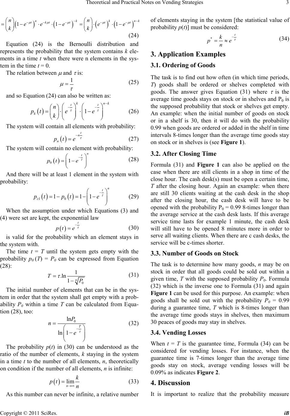
−
−
−
− −−

=−⋅⋅−=




⋅−⋅−=−⋅−
 
 
 

Theoretical and Practical Notes on Vending Strategies
3
( )( )()( )
111
nkk nk
t ktttt
nn
ee eee
kk
µµ µµµ
−−
−− −−−

=−⋅⋅−= ⋅⋅−


(24)
Equation (24) is the Bernoulli distribution and
represents the probability that the system contains k ele-
ments in a time t when there were n elements in the sys-
tem in the time t = 0.
The relation between
µ and τ is:
1
µτ =
(25)
and so Equatio n (24) can also be written as:
( )
1
k nk
tt
k
n
pt ee
k
ττ
−
−−  

= ⋅⋅−
 

 

 
(26)
The system will contain all elements with pr obability:
( )
t
n
n
pt e
τ
−
=
(27)
The system will contain no element with probability:
( )
01
n
t
pt e
τ
− 
= −



(28)
And there will be at le ast 1 element in the s ystem with
probability:
( )( )
10
1 11
n
t
p tpte
τ
−
≥

=− =−−



(29)
When the assumption under which Equations (3) and
(4) were set are kept, the expo nential law
( )
t
pt e
τ
−
=
(30)
is valid for the probability which an element stays in
the s ys tem with.
The time t = T until the system gets empty with the
probability p0 (T) = P0 can be expressed from Equation
(28):
0
1
ln1
n
T. P τ =−
(31)
The initial number of elements that can be in the sys-
tem in orde r that the sys tem shall get e mpty with a p rob-
ability P0 within a time T can be calculated from Equa-
tion (28), too:
0
ln
ln 1
T
P
n
e
τ
−
=
−



(32)
The probability p(t) in (30) can be understood as the
ratio of the number of elements, k staying in the system
in a time t to the number of all elements, n, theoretically
on condition i f the number of all e lements, n is infinite:
( )
lim
n
k
pt n
→∞
=
(33)
As t hi s number can ne ver be infini t e, a relative number
of ele ments sta ying i n the s ystem [the statistica l value of
probability p(t)] must be considered :
t
*k
pe
n
τ
−
= ≈
(34)
3. Application Examples
3.1. Ordering of Goods
The task is to find o ut ho w o ften (in which time per iods,
T) goods shall be ordered or shelves completed with
goods. The answer gives Equation (31) where
τ is the
aver age time goo ds sta ys on s tock o r in she lves a nd P 0 is
the supposed probability that stock or shelves get empty.
An example: when the initial number of goods on stock
or in a shelf is 30, then it will do with the probability
0.99 when goods are ordered or added in the shelf in time
intervals 8-ti mes lo nger t han the a verage t ime go ods sta y
on stock or in shelves is (see Fig ure 1).
3.2. After Closing Time
Formula (31) and Figure 1 can also be applied on the
case when there are still clients in a shop in time of the
close hour. The cash desk(s) must be open a certain time,
T after the closing hour. Again an example: when there
are still 30 clients waiting at the cash desk in the shop
after the closing hour, the cash desk will have to be
opened with the probability P0 = 0.99 8-times longer tha n
the average service at the cash desk lasts. If this average
service time lasts for example 1 minute, the cash desk
will still have to be opened 8 minutes more in order to
serve all waiting clients. When there are c cash desks, the
service will be c-times shorter .
3.3. Number of Goods on Stock
The task is to determine how many goods, n may be on
stock in order that all goods could be sold out within a
given time, T with the supposed probability P0. Formula
(32) which is the inverse one to Formula (31) and again
Figure 1 can be used for this purpose. An exa mple: when
goods shall be sold out with the probability P0 = 0.99
during a guarantee time, T which is 8-times longer than
the average time goods stays in shelves, then maximum
30 peaces of goods may stay in shelves.
3.4. Vending Losses
When t = T is the guarantee time, Formula (34) can be
considered for vending losses. For instance, when the
guarantee time is 7-times longer than the average time
goods stay on stock, average vending losses will be
0.09% as indicates Figure 2.
4. Discussion
It is important to realize that the probability measure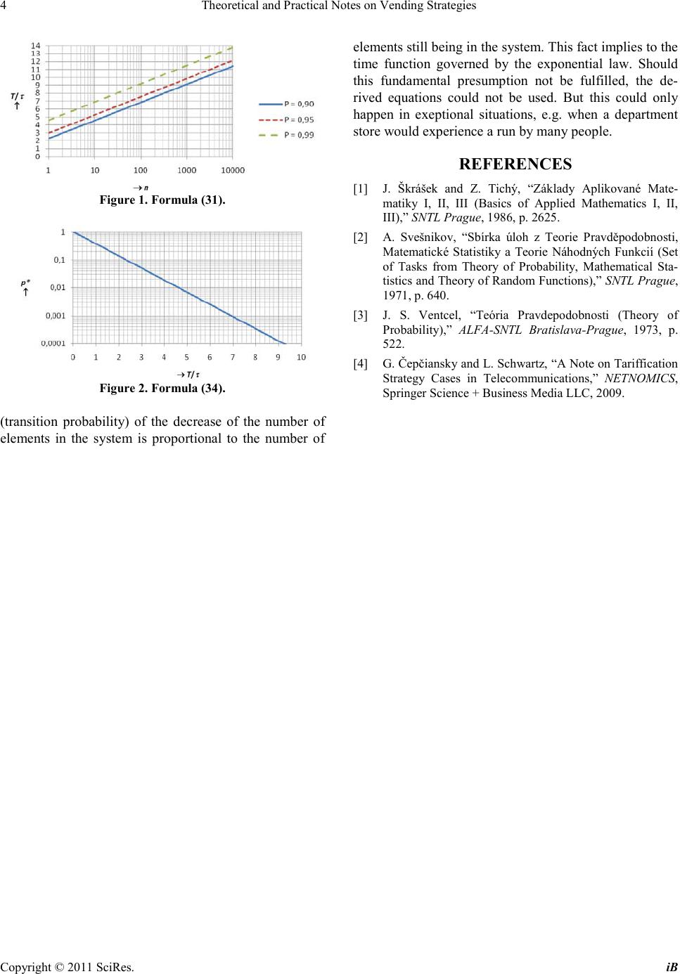

Theoretical and Practical Notes on Vending Strategies
4
Figure 1. Formula (31).
Figure 2. Formula (34).
(transition probability) of the decrease of the number of
elements in the system is proportional to the number of
elements still be ing in the syste m. This fact i mplies to the
time function governed by the exponential law. Should
this fundamental presumption not be fulfilled, the de-
rived equations could not be used. But this could only
happen in exeptional situations, e.g. when a department
store would experience a run by many people.
REFERENCES
[1] J. Škrášek and Z. Tichý, “Základy Aplikované Mate-
matiky I, II, III (Basics of Applied Mathematics I, II,
III),” SNTL Prague, 1986, p. 2625.
[2] A. Svešnikov, “Sbírka úloh z Teorie Pravděpodobnosti,
Matematické Statistiky a Teorie Náhodných Funkcií (Set
of Tasks from Theory of Probability, Mathematical Sta-
tistics and Theory of Random Functions),” SNTL Prague,
1971, p. 640.
[3] J. S. Ventcel, “Teória Pravdepodobnosti (Theory of
Probability),” ALFA-SNTL Bratislava-Prague, 1973, p.
522.
[4] G. Čepčiansky and L. Schwartz, “A Note on Tariffication
Strategy Cases in Telecommunications,” NETNOMICS,
Spri nger Science + Business Media LLC, 2009.