Open Journal of Forestry
2014. Vol.4, No.1, 42-48
Published Online January 2014 in SciRes (http://www.scirp.org/journal/ojf) http://dx.doi.org/10.4236/ojf.2014.41008
A Comparison of Selected Parametric and Non-Parametric
Imputation Methods for Estimating Forest
Biomass and Basal Area
Donald Gagliasso1, Susan Hummel2, Haile mariam Temesgen1
1Department of Forest Engineering, Resources and Management, Oregon State University, Corvallis, USA
2USDA Forest Service, Goods, Services, and Values Program, Portland Forest Sciences Laboratory, US Forest
Service, Pacific Northwest Research Station, Portland, USA
Received October 19th, 2013; revised November 21st, 2013; accepted December 23rd, 2013
Copyright © 2014 Donald Gagliasso et al. This is an open access article distributed under the Creative Com-
mons Attribution License, which permits unrestricted use, distribution, and reproduction in any medium, pro-
vided the original work is prop erly cited. In accordance of the Creative Commons Attributio n License all Copy-
rights © 2014 are reserved for SCIRP and the owner of the intellectual property Donald Gagliasso et al. All
Copyright © 2014 a re guarded by law and by SCIRP as a guardian.
Various methods have been used to estimate the amount of above ground forest biomass across land-
scapes and to create biomass maps for specific stands or pixels across ownership or project areas. Without
an accurate estimation method, land managers might end up with incorrect biomass estimate maps, which
could lead them to make poorer decisions in their future management plans. The goal of this study was to
compare various imputation methods to predict forest biomass and basal area, at a project planning scale
(<20,000 acres) on the Malheur National Forest, located in eastern Oregon, USA. We examined the pre-
dictive performance of linear regression, geographic weighted regression (GWR), gradient nearest neigh-
bor (GNN), most similar neighbor (MSN), random forest imputation, and k-nearest neighbor (k-nn) to es-
timate biomass (tons/acre) and basal area (sq. feet per acre) across 19,000 acres on the Malheur National
Forest. To test the different methods, a combination of ground inventory plots, light detection and ranging
(LiDAR) data, satellite imagery, and climate data was analyzed, and their root mean square error (RMS E)
and bias were calculated. Results indicate that for biomass prediction, the k-nn (k = 5) had the lowest
RMSE and least amount of bias. The second most accurate method consisted of the k-nn (k = 3), followed
by the GWR model, and the random forest imputation. For basal area prediction, the GWR model had the
lowest RMSE and least amount of bias. The second most accurate method was k-nn (k = 5), followed by
k-nn (k = 3), and the random forest method. For both metrics, the GNN method was the least accurate
based on the ranking of RMSE and bias.
Keywords: Gradient Nearest Neighbor; Most Similar Neighbor; K-Nearest Neighbor; Random Forest;
Geographic Weighted Regression; Biomass; LiDAR
Introduction
Estimates of forest biomass and basal area provide critical
information for quantifying the amount of carbon sequestrated,
making management decisions, designing processing plants,
guiding decisions among conflicting land uses, and establishing
and quantifying wildlife habitats. To meet national and interna-
tional negotiations and reporting requirements, forest manage-
ment plans require local inventory data on biomass, vegetation,
site productivity, carbon, and other resources. The data must be
intensive enough to include structural variables relevant to
biomass and carbon projections and extensive enough to cover
hundreds to thousands of acres, but not be too expensive to
collect.
Recognition of the widespread need for cost-effective, local
inventory data that spans large regions has led to new methods
for imputing plot data to sites without data and then generating
maps of regional biomass and productivity. One imputation
method is the Gradient Nearest Neighbor (GNN). Vegetation
maps created using GNN now figure prominently into intera-
gency (Oregon Department of Forestry, USDI Bureau of Land
Management, and USDA Forest Service) analysis and planning
efforts across the Pacific Northwest. In addition, they are being
used to estimate the supply of woody biomass available to pro-
posed energy facilities and in regional conservation planning.
Other techniques that use imputation, including K-NN (k-
Nearest Neighbor), are used in parts of the Pacific Northwest.
Both GNN and K-NN are used to derive forest biomass and
basal area maps. For example, one can combine satellite im-
agery with data from field plots and impute a raster dataset
showing a continuous map of biomass and basal area across the
landscape (Ohmann & Gregory, 2002).
GNN maps are created by using a multivariate model that
integrates field plot data with satellite imagery and current
mapped environmental data. GNN uses the nearest neighbor, or
shortest distance, from a point to the nearest plot in predictor
space to generate volume and basal area estimates that are then
42

D. GAGLIASSO ET AL.
related to a specific timber type. The distance is measured by
creating a weight matrix derived by canonical correspondence
analysis (Ohmann & Gregory, 2002). Similarly, MSN maps are
created using a model that also integrates field plot data with
satellite imagery. In contrast, MSN uses a canonical correlation
analysis to derive a similarity function, with selected response
variables, to impute data to pixels where no ground plots exist
(Moeur & Stage, 1995). The k-MSN method uses the same
methods as MSN, but takes an average of the k nearest neigh-
bor of plots. The Random Forest (RF) imputation method
creates a classification matrix and regression tree in order to
find similarities between the explanatory and response variables
(Crookston & Finley, 2008).
Nearest neighbor imputations have been used to perform
multivariate analyses of forested landscapes by associating
variables of interest (e.g. ground data) to aerial data (Temesgen
et al., 2003), satellite imagery (Eskelson et al., 2009a), and light
detection and ranging (LiDAR) data (Hudak et al., 2008;
Goerndt et al., 2010). Different analyses have ranked the me-
thods and data sources differently in different forest types. For
example, in north-central Idaho, Hudak et al. (2008) found that
the RF method performed best at predicting plot level estimates
such as basal area and tree density. In Finland, Maltamo et al.
(2006) compared k-MSN imputations for plot and stand level
volume estimates and found that aerial-laser scanner data re-
sulted in better estimates than using aerial photo imagery esti-
mates and, when laser and photo data were used together, the
resulting root mean square error improved again. Eskelson et al.
(2009a) found that the RF method performed best when com-
pared to the moving average, weighted moving average, and
MSN and GNN imputation methods.
Parametric methods are an alternative to the nearest neighbor
imputation methods that can be used to estimate selected va-
riables of interest (Fotheringham et al., 2002; Wang e t al., 2005;
Salas et al., 2010; Crow & Schlaegel, 1988). Linear and non-
linear models have been used for this purpose in previous stu-
dies (Wang et al., 2005; Nelson et al., 2004). Another option is
geographic weighted regression (GWR), which takes a global
regression model and localizes it to a specific area and allows
relationships between the explanatory and response variables to
account for spatial variations, by including a weighting function
in the regression model Fotheringham et al. (2002).
Wang et al. (2005) developed an ordinary least squares (OLS)
model, a spatial lag model, and a GWR model to analyze the
amount of net primary production (NPP) in forest ecosystems
across China. They used predictor variables that included forest
stand locations, forest inventory data, and remotely sensed data.
The authors found that the GWR model was superior to both
the OLS model and the spatial lag model in predicting NPP.
Salas et al. (2010) modeled tree diameter using forest inven-
tory and ancillary data. The models that the authors compared
were OLS, generalized least squares (GLS), GWR, and linear
mixed effects (LME). The authors used aerial LiDAR data and
forest inventory plots to estimate diameter at breast height on
individual trees in Norway. They found that the most precise
approach was LME and GWR performed better than both the
OLS and GLS.
Airborne LiDAR Scanner (ALS)
When current field inventory data are insufficient to achieve
desired precision, a common practice is to increase the number
of ground plots to measure the forest inventory. This can be
costly and time-consuming. A newer practice would be to use
LiDAR data. LiDAR is a tool that forestry researchers and pro-
fessionals are increasingly using to improve estimates of forest
inventory attributes; the cost may be comparable to traditional
ground inventory data collection (Hummel et al., 2011).
LiDAR data are becoming a useful tool in obtaining large
amounts of forest inventory data due to its precision and rela-
tive ease of ground truthing. Ground truthing LiDAR data consist
of randomly locating plots across the landscape, measuring the
trees on the plot, a nd georeferencing the trees so that t hey can be
located in the LidAR data set for crown delineation (Wulder et al.,
2008). LiDAR datasets can be used to describe large areas of
forested landscape at one time.
Nelson et al. (2004) used LiDAR to estimate the amount of
biomass and carbon in the state of Delaware. The authors used
parallel flight lines 4 kilometers apart to measure the merchan-
table forest volume, biomass and above ground carbon. Using
four explicitly linear models the authors predicted merchantable
forest volume and above ground biomass across the state. The
authors found that merchantable volume estimates were within
22% of US Forest Service (USDA FS) estimates county wide
and 15% statewide. Additionally, the authors found that their
biomass estimates were within 22% of USDA FS estimates
county wide and 20% statewide. The USDA FS estimates were
based on FIA volume and biomass estimates at the county and
state level.
Næsset (2004) reported on the first Nordic stand-based forest
inventory using LiDAR. The author predicted six stand va-
riables from LiDAR data: mean tree height, dominant height,
mean diame ter, basal area, ste m volume and stem number . Plot
and tree level data were collected, including tree diameter at
breast height (dbh), and tree height. With the plot data the au-
thor calculated: mean height, dominant height, mean diameter
by basal area, plot basal area, number of trees per hectare, and
total plot volume. The author found that 85% - 95% of the va-
riability was explained by the regression models for mean
height and dominant height. Additionally, 72% - 85% of the
variability was explained by the regression models for basal
area and stand volume and 49% - 63% of the variability was
explained by the regression models for mean diameter and stem
number. Validation of the models revealed the mean differ-
ences between the ground truth data and the predicted values
were statistically significant in 5 of 24 cases.
In this article, we examine the performance of four parame-
tric and two non-parametric methods for estimating the amount
of standing tree biomass and basal area at a pixel level, across
the a site on the Malheur National Forest, in Eastern Oregon,
US: Gradient Nearest Neighbor (GNN), Most Similar Neighbor
(MSN), k-MSN, and the Random Forest (RF) nearest neighbor
methods, and linear regression and geographic weighted re-
gression. The different methods were assessed for their accura-
cy by comparing measured ground plot values to model esti-
mates.
Materials and Methods
Project Site
The project site consists of 19,904 acres on the Malheur Na-
tional Forest, located in the Blue Mountains of eastern Oregon
(Figure 1), called the Damon project si te.
OPEN ACCESS 43

D. GAGLIASSO ET AL.
Figure 1.
LiDAR datasets on the Malheur National Forest.
Airborne LiDAR Scanner
The LiDAR data were collected during the fall of 2007 by
Watershed Sciences, Inc. The LiDAR was acquired with a Lei-
ca ALS50 Phase II device mounted on a Cessna Caravan 208B.
The scan angle was ±14˚ from nadir with an intended pulse
density of ≥4 pulse per square meter. The Leica ALS50 Phase
II laser system is designed for up to four returns per pulse, and
all laser returns were processed for the dataset. The actual pulse
density was 6 pulses per square meter for the Damon site.
Ground Data
We had field data from three sources. Previously collected
ground data consisted of United States Forest Service (USDA
FS) stand exams from 2008 and current vegetation survey
(CVS) plots measured between 1998 and 2007 (US Forest Ser-
vice). The stand exams and CVS plots were grown forward to
2009 with the Forest Vegetation Software (FVS) for the Blue
Mountain region (Keyser & Dixon, 2008). Eight additional
cluster plots were measured during the summer of 2009 (Table
1).
The USDA FS stand exam data consist of 98 plots that were
measured in the summer of 2008. Stand Exam plots are a nested
plot design that consists of a variable radius plot for large trees
and fixed radius plots for small trees and seedlings. A profes-
sional forester from the USDA FS went back and re-measured
the plot so that a 1/10th acre fixed plot was used for the large
trees, instead of the previously measured variable radius plot
design. These data were analyzed internally by the Forest Ser-
vice within their plot compiler.
Table 1.
Number of plots in Damon site.
Source Number of Plots
USFS Current Vegetation System 10
USFS Stand Exams 98
Summer 2009 8
CVS plot data were supplied by the USDA FS. CVS are
permanent forest inventory plots in Region 6 (Pacific North-
west) of the USDA FS. Each plot is re-measu red on ce every ten
years. Within this study site, CVS plots are on a 1.7 mile sys-
tematic grid. The plots consist of a 2.47-acre circular plot with
5 sub-plots. Each sub-plot is a set of 3 plo ts: 1) 1/5.3-acre plot,
2) 1/24-acre plot, and 3) 1/100-acre plot. Each plot has set cri-
teria for which data should be collected and recorded, including
live and dead tree measurements, down woody debris, shrub
and understory components, and general geographical and slope
position information of the plot (US Forest Service, 2001).
Recent research has shown that stratifying the landscape us-
ing LiDAR data is an efficient and effective way to group the
landscape into similar forest type and structure for further anal-
ysis (Sullivan, 2008; Koch et al., 2009; Mustonen et al., 2008).
Accordingly, forested stands were delineated using differences
in height and canopy closure characteristics. Percent canopy
closure, 25th and 75th height percentiles were used following the
process outlined by Sullivan (2008), stand delineations were
created using two software packages, FUSION (McGaughey,
2009) and Spring (Câmara et al., 1996). The latter is a user-
based classification software package. For this study, the stand
density index (SDI) of forest service stand exam plots measured
in 2006 was used for the training data of the user-based classi-
fication process.
The 8 cluster plots measured during the summer of 2009
consisted of a linear cluster (CLUS) of plots of four rectangular
fixed radius subplots. Moisen et al. (1994) showed that linear
clusters of plots was a cost efficient way of distributing forest
inventory plots for assessing map accuracy, while accounting
for spatial autocorrelation. The advantage of using a CLUS
design is less cost in traveling to each plot as compared to a
random design, while the disadvantage for CLUS is that there is
more potential for spatial autocorrelation. Due to availability of
previously collected inventory data we opted to use the cluster
design to sample more ground area with our limited resources
without sacrificing the total number of plot estimates. Our li-
near clusters consisted of four 1/10-acre rectangular fixed area
plots. In order to assure a random sample, a grid of 1/10-acre
plots was placed over the project area and a random location
was selected based on the plot allocation information previous-
ly computed. The other three plots were located by obtaining a
random azimuth in one of the four cardinal directions, from the
first plot center, and installing the three additional plots in a
linear fashion.
Each tree in a plot was measured for diameter-at-breast
height (DBH), species, and crown dominance (dominant,
co-dominant, intermediate, or over-topped). A tree was meas-
ured if it was 4.5 feet tall or larger. The first, third and fifth tree
per species per plot were measured for height, crown diameter,
and crown ratio. Crown diameter was measured by taking a
random azimuth and measuring the diameter of the crown at
44

D. GAGLIASSO ET AL.
that azimuth, then taking the diameter of the crown perpendi-
cular to the first measurement and averaging the two. Dead
trees and snags, greater than five inches DBH were measured
for DBH and height. All trees with broken tops were measured
for height.
Ground data were collected on a TDS Ranger handheld
computer, with the USDA FS Stand Exam software. Missing
heights were estimated with localized height-diameter equa-
tions for the Blue Mountains as described in stand exam proto-
cols (USDA FS, 2001).
Data Compilation
Total standing tree woody biomass (tons per acre) was esti-
mated for each ground inventory plot. In this study, standing
tree woody biomass is defined as the biomass of the bole, bark,
and branches of the all standing dead and live trees that are
greater than or equal to 4.5 feet tall. Volume and biomass esti-
mates were calculated using the USDA FS Forest Inventory
Analysis (FIA) equations cubic volume, including top and
stump, and biomass equations for the Blue Mountains (US DA
FS 2001). All results found in this study assume that the USDA
FS FIA equations are true and that the underlying assumptions
of the volume and biomass models are applicable to this study
area.
LiDAR data were processed with FUSION (McGaughey,
2009). Raw LiDAR data files were clipped to each individual
ground inventory plot and attributes such as a digital elevation
model (DEM), height percentiles, and their variances were
obtained. Additionally, using the GridMetrics batch processing
tool these same estimates were obtained for all other areas
within the study area. Percent cover, percent slope, aspect, and
elevation of each plot were found using the LiDAR derived
DEM.
Landsat Thematic Mapper (TM) data was downloaded from
the United States Geological Survey Global Visualization
(GloVis) website for the entire project area. The normalized
difference vegetation index (ndvi) was calculated using bands
three and four.
Climate data from the DAYMET website (Thornton, 2003)
was downloaded for the entire project area. Variables of interest
consisted of: average daily maximum temperature, average
daily minimum temperature, average temperature, number of
growing degree days, number of frost days, and total precipita-
tion. All variables were merged into one large table on a 20 ×
20 meter pixel grid. Additionally, each of the ground inventory
plots was added as separate rows to the table.
Statistical Analysis
For this study, explanatory variables were determined for the
nearest neighbor imputations and geographic weighted regres-
sion, by implementing an all subsets stepwise regression tech-
nique, as outlined by Goerndt et al. (2010), using the regsub-
sets() function within the leaps package (R Development Core
Team, 2011). This tool returns the best fitting linear models
according to the Bayesian information criteria (BIC).
Using the eight independent variables found by the best fit-
ting linear model, a geographic weighted regression (GWR)
model was fit using the gwr tool within the spgwr R-package.
Before a back transformation of the natural log biomass esti-
mate was performed, a bias-correction factor of 0.5 times the
mean square error was added to the estimates (Baskerville,
1972; Goerndt et al., 2010). Most similar neighbor (MSN),
gradient nearest neighbor (GNN), k-nearest neighbor (k-MSN),
and random forest (RF) were performed using the yai and im-
pute tools within the yaImpute (Crookston & Finley, 2008)
R-package.
Each model was assessed using the 116 plots located within
the study area. We used root mean square error (RMSE) and
bias to evaluate the models. These values were estimated using
a leave one out plot cross-validation. The root mean square
error (Equation (1)) and bias (Equation (2)) were calculated
using the following:
( )
2
1
ˆ
n
ii
i
YY
RMSE n
=
−
=∑
, (1)
( )
1
ˆ
n
ii
i
YY
bias n
=
−
=∑
, (2)
where Yi is the observed value,
ˆ
i
Y
is the imputed estimate,
and n is the sample size (number of plots).
Results
The best linear model, for estimating biomass (tons per acre)
on a plot included the following explanatory variables: the
minimum value from the LiDAR height percentile profile
(Min_Elev), 80th percentile value of the height profile from the
LiDAR data (P80), the longitudinal location of the plot
(UTM_Y), the reflective property value of Landsat TM band 2
(LandsatB2), Normalized Difference Vegetation Index (ndvi),
18-year average daily minimum temperature (MinTemp),
18-year average of the number of growing degree days (Deg-
Day), a nd the 18-year average of the annual precipitation (Tot-
Precip). The results of this linear model can be seen in Table
2.
The best fitting linear model, for estimating basal area per
acre included the following variables: the standard deviation of
all LiDAR returns on the plot (StdDev), the 95th percentile val-
ue of the height profile from the LiDAR data (P95), and the
reflective property value from Landsat TM band 5 (LandsatB5).
The results from this linear model can be seen in Table 3.
The inventory plots ranged in cover type, from non-forest
meadows, to highly dense pine forests. Biomass measured on
the inventory plots ranged from zero tons per acre to 103.7 tons
per acre, with a standard deviation of 15.9 tons per acre. The
basal area of the inventory plots ranged from zero square feet
per acre to 248.7 square feet per acre, with a standard deviation
of 55.6 square feet per acre (Table 4).
Nearest neighbor imputations rely on explanatory variables
being correlated with the response variables. Thus, the higher
the correlation coefficient the better the imputation model
should perform. The highest correlation between the predictor
variables and biomass per acre comes from the LiDAR derived
P80 variable, a correlation coefficient of 0.44 (Table 5).
The highest coefficient in the basal area prediction methods
was the P95 variable, correlation coefficient of 0.69 (Table 6).
The RMSE and bias for the nearest neighbor and OLS re-
gressions for biomass (tons per acre) and basal area (square feet
per acre) models are reported in Tables 7 and 8, respectively.
For the biomass prediction, the k-MSN, k = 5, has the lo west
RMSE and least amount of bias. The second most accurate
method consisted of the k-MSN, k = 3, followed by the GWR
OPEN ACCESS 45

D. GAGLIASSO ET AL.
model and the RF imputation. The GNN method was the least
accurate (Table 7). For basal area prediction, the GWR model
has the lowest RMSE and the least amount of bias. The second
most accurate method was k-MSN, k = 5, followed by the
k-MSN, k = 3 and then random forest. The GNN method was
again th e least accu r ate (Table 8).
Table 2.
Coefficients and standard errors for linear regression model for ln(biomass) in tons per acre.
80th percentile value from the LiDAR height profile 0.0525 0.0165
UTM northing −0.0003 0.0000
Reflec t i ve property of Landsat TM band 2 −0.1705 0.0411
Normalized Difference Vegetation Index −6.382 1.359
18 year average of the daily minimum temperature 5.052 0.2276
18 year average of the number of grow ing degree days 0.0329 0.0049
18 year average of the annual precipitation 1.231 0.1741
Table 3.
Coefficient and standard errors for linear regression model for basal area (ft2 per acre).
Variable Coefficient SE
Intercept 50.12 22.32
Standard de vi ation of al l LiDAR ret ur ns on the plot −27.79 5.212
95th percentile value from the LiDAR height profile 11.88 1.634
Reflec t i ve property of Landsat TM band 5 −0.7082 0.1908
Table 4.
Basic statistics of explanatory and response variables1.
Biomass (tons per acre) Explanatory variables
units Min_Elev
meters P80 meters UTM_Y LandsatB2 µm ndvi MinTemp celsius DegDay degree days TotPrecip cm
Minimum 1.00 0.00 4882625.7 23.0 0.2 −4.2 1895.7 46.2
Maximum 4.42 33.9 4901661.6 39.0 0.7 −2.2 2541.2 64.5
Mean 1.14 14.5 4890903.5 27.8 0.4 −2.9 2298.9 54.0
Median 1.02 14.8 4888069.0 27.0 0.4 −2.8 2312.5 53.9
Standard Deviation 0.38 6.34 6759.8 3.5 0.1 0.5 168.0 4.2
Basal Area Explanatory Variables
units Biomass
tons per acre Basal Area square feet per acre StdDev meters P95 meters Landsat B5 µm
Minimum 0.0 0.0 0.0 0.0 47.0
Maximum 103.7 248.7 13.6 42.6 134.0
Mean 8.9 79.3 4.7 18.2 80.0
Median 2.9 77.1 4.4 18.2 75.0
Standard
Deviation 15.9 55.6 2.3 7.7 19.8
1Min_Elev = Minimum value of the LiDAR percentile height profile. P80 = 80th percentile of the Li DAR h eight profile. UTM_Y = UTM no rt hin g coo rdi nate. LandsatB2 =
reflective property of Landsat TM band 2. Ndvi = normalized difference vegetation index. MinTemp = 18-year average of the minimum temperature. DegDay = 18 year
average of the number of degree days. TotPrecip = 18-year average of the annual precipitation. StdDev = standard deviation of all LiDAR values on the plot. P95 = 95th
percentile of the L iDAR hei ght profile. LandsatB5 = reflective property of Landsat TM band 5.
46

D. GAGLIASSO ET AL.
Table 5.
Correlation coefficients of biomass vs. selected predictor variables2.
ln_Biomass ln_BA Min_Elev P80 UTM_Y LandsatB2 ndvi MinTemp DegDay
ln_BA 0.4339
Min_Elev −0.2310 −0.0870
P80 0.4368 0.5303 −0.0827
UTM_Y −0.3135 −0.1858 0.1243 −0.2442
LandsatB2 −0.3320 −0.4832 0.1873 −0.5834 0.4484
ndvi −0.0516 0.1673 −0.0568 0.3494 −0.0614 −0.5555
Min Temp 0.0321 −0.0374 0.2089 −0.0473 0.4424 0.2309 −0.2012
DegDay −0.1544 −0.0488 0.1485 −0.1336 0.4563 0.1331 −0.1158 0.5835
TotPrecip 0.1158 −0.0064 −0.1164 0.0742 −0.1848 0.0158 0.1085 −0.4904 −0.9529
2Min_Elev = Minimum value of the LiDAR percentile height profile. P80 = 80th percentile of the Li DAR h eight profile. UTM_Y = UTM no rt hin g coo rdi nate. LandsatB2 =
reflective property of Landsat TM band 2. Ndvi = normalized difference vegetation index. MinTemp = 18-year average of the minimum temperature. DegDay = 18 year
average of the number of de gree days. TotPrecip = 18-year average of the annual precipitation.
Table 6.
Correlation Coefficients of basal area vs. selected predictor variables.
Biomass per acre Basal area per acre Standard De vi ation of
LiDAR returns 95th percentile value of LiDAR height profile
Basal area per acre 0.4372
Standard Deviation of L i DAR returns 0.1691 0.5749
95th percentile value of
LiDAR height profile 0.1883 0.6870 0.9651
Reflective property of
Landsat TM band 5 −0.2282 −0.6225 −0.4757 −0.5477
Table 7.
RMSE and bias for estimating biomass (tons/acre) by selected method.
Model RMSE Bias
Linear regression 12.7 −2.41
Geographic Weighted Regression 11.6 −0.67
Gradient Nearest Neighbor 16.31 −0.008
Most Similar Neighbor 13.96 −0.08
Random Forest 12.22 −1.87
k-MSN (k = 3) 11.53 0.24
k-MSN (k = 5) 11.24 −0.004
Discussion
Substantial differences were found among the predictive ab-
ilities of the strategies examined to predict forest biomass and
basal area. As a result, the seemingly divergent parametric and
non-parametric approaches resulted in different predictions.
GWR outperformed the other methods in terms of accuracy and
precision when predicting basal area per acre. This might be
ascribed to GWR’s ability to localize the relation between the
response variable and covariate in both the geographical and
feature and variable space.
Table 8.
RMSE and bias for estimating basal area (ft2/acre) by selected method.
Model RMSE Bias
Linear regression 33.15 0.0029
Geographic Weighted Regression 33.08 0.0082
Gradient Nearest Neighbor 58.65 −4.79
Most Similar Neighbor 50.99 0.13
Random Forest 39.03 2.82
k-MSN (k = 3) 39.02 0.67
k-MSN (k = 5) 38.62 0.71
Possible reasons for GNN performing poorly, compared to
the other methods, include the small size of the project site
compared to previous uses of the GNN method (Ohmann &
Gregory, 2002) and the explanatory variables’ lack of high
correlation with the response variables. The GWR method may
perform better than the non-parametric approaches due to only
predicting one response variable, biomass. In contrast, the
nearest neighbor methods are predicting both biomass and basal
area simultaneously. Therefore, GWR may be sufficient for the
estimation of biomass per acre if that is the only variable of
interest; while, the nearest neighbor imputations are preferred
OPEN ACCESS 47

D. GAGLIASSO ET AL.
when multiple response variables of interest are present in the
analysis. When predicting a single variable, Eskelson et al.
(2009b) reported that parametric methods resulted in better
performance than non-parametric methods.
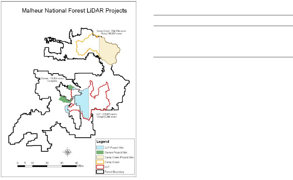
The results of this study suggest that the current method be-
ing used to implement forest management activities on the
Malheur National Forest, MSN, may not be the best method to
predict total standing tree woody biomass. Instead, the k-MSN
or RF method may be preferable, particularly if multiple re-
sponse variables are important to consider. In contrast, if users
are only interested in a single response variable, total standing
tree biomass, GWR appears more suitable.
REFERENCES
Baskerville, G. L. (1972). Use of logarithmic regression in the estima-
tion of plant biomass. Canadian Journal of Fores try, 2, 49-53.
http://dx.doi.org/10.1139/x72-009
Câmara, G., Souza, R., Freitas, U., & Garrido, J. (1996). SPRING:
Integrating remote sensing and GIS by object-oriented data modeling.
Computers and Gr aphics, 20, 395-403.
http://dx.doi.org/10.1016/0097-8493(96)00008-8
Crookston, N. L., & Finley, A. O. (2008). yaImpute: An R package for
kNN imputation. Journal of Statistical Software, 23, 1-16.
Crow, T. R., & Schlaegel, B. E. (1988). A guide to using regression
Equations for estimating tree biomass. Northern Journal of Applied
Forestry, 5, 15-22.
Eskelson, B. N. I., Temesgen , H., & Barrett, T. M. (2009a). Estimating
current forest attribu tes from paneled inventory data using plo t-level
imputation: A study from the Pacific Northwest. Forest Science, 5,
64-71.
Eskelson, B. N. I., Temesgen, H., & Barrett, T. M. (2009b). Estimating
cavity tree and snag abundance using negative binomial regression
models and nearest neighbor imputation methods. Canadian Journal
of Forest Research, 39, 1749-1765.
http://dx.doi.org/10.1139/X09-086
Fotheringham, A. S., Brunsdon , C., & Charlton, M . (2002). Geograph-
ically weighted regression: The analysis of spatially varying rela-
tionships. Chichester, Hoboken, NJ: Wiley.
Goerndt, M. E., Monleon, V. J., & Temesgen, H. (2010). Relating
forest attributes with area - and tree-based lig ht detection an d ranging
metrics for Western Oregon. Western Journal of Applied Forestry,
25, 105-111.
Hudak, A. T., Crookston, N. L., Evans, J. S., Hall, D. E., & Falkowski,
M. J. (2008). Nearest neighbor i mputation of species-level, plo t-scale
forest structure attributes from LiDAR data. Remote Sensing of En-
vironment, 112, 2232-2245. Corrigendum: (2009). Remote Sensing of
Environment, 113, 289-290.
http://dx.doi.org/10.1016/j.rse.2008.08.006
Hummel, S., Hudak, A. T., Uebler, E. H., Falkowski, M. J., & Megown,
K. A. (2011). A comparison of accuracy and cost of LiDAR versus
stand exam data for landscap e management on the Malheur Nation al
Forest. Journal of Forest r y, 109, 267-273.
Keyser, C. E., & Dixon, G. E. (2008). Blue Mountains (BM) variant
overview—Forest vegetation simulator. Internal Rep., Fort Collins,
CO: US Department of Agriculture, Forest Service, Forest Manage-
ment Service Center. (revised February 3, 2010)
Koch, B., Straub, C., Dees, M., Wang, Y., & Weinacker, H. (2009).
Airborne laser data for stand delineation and information extraction.
International Journal of Remote Sensing, 30, 935-963.
http://dx.doi.org/10.1080/01431160802395284
Maltamo, M., Malinen, J., Packalén, P., Suvanto, A., & Kangas, J.
(2006). Nonparametric estimation of stem volume using airborne la-
ser scanning, aerial photography, and stand-register data. Canadian
Journal of Forest Research, 36, 426-436.
http://dx.doi.org/10.1139/x05-246
McGaughey, R. J. (2009). FUSION/LDV: Software for LIDAR data
analysis and visualization, Version 2.9. USDA FS.
http://www.fs.fed.us/eng/rsac/fusion/
Moeur, M., & Stage, A. R. (1995). Most similar neighbor: An improved
sampling inference procedure for natural resource planning. Forest
Science, 41, 337-359.
Moisen, G. G., Edwards J r., T. C., & Cutler, D. R. (1994). Spatial sam-
pling to assess classification accuracy of remotely sensed data. In J.
Brunt, S. S. Stafford, & W. K. Michener (Eds.), Environmental in-
formation management and analysis: Ecosystem to glob al scales (pp.
161-178). Philadelphia, PA: Taylor and Francis.
Mustonen, J., Packalén, P., & Kang as, A. (2008). Automatic segmenta-
tion of forest stands using canopy height model and aerial photo-
graph. Scandinavian Journal of For est Research, 23, 534-545.
http://dx.doi.org/10.1080/02827580802552446
Ohmann, J. L., & Gregory, M. J. (2002). Predictive mapping of forest
composition and structure with direct gradient analysis and nearest-
neighbor imputation in coastal Oregon, U.S.A. Canadian Journal of
Forest Research, 32, 725-741. http://dx.doi.org/10.1139/x02-011
Næsset, E. (2004). Accuracy of forest inventory using airborne laser
scanning: Evaluating the first Nordic full-scale operation project.
Scandinavian Journal of Fores t Research, 19, 554-557.
http://dx.doi.org/10.1080/02827580410019544
Nelson, R., Short, A., & Valenti, M. (2004). Measuring biomass and
carbon in Delaware using an airborne profiling LiDAR. Scandina-
vian Journal of Forest Research, 19, 500-511.
http://dx.doi.org/10.1080/02827580410019508
R Development Core Tea m (2011). R: A language and environment for
statistical computing. Vienna: R Foundation for Statistical Compu-
ting. http://www.R-project.org/
Salas, C., Ene, L., G regoire, T. G., Næsse t, E., & Gobakken, T. (2010).
Modelling tree diameter from airborne laser scanning derived va-
riables: A comparison of spatial statistical models. Remo te Sen sin g of
Environment, 114, 1277-1285.
http://dx.doi.org/10.1016/j.rse.2010.01.020
Sullivan, A. (2008). LIDAR based delineation in forest stands. Master’s
Thesis, Seattle, WA: University of Was hington.
Temesgen, H., LeMay, V. M., Marshall, P. L., & Froese, K. (2003).
Imputing tree-lists from aerial attributes for complex stands of
south-eastern British Columbia. Forest Ecology and Management,
177, 277-285. http://dx.doi.org/10.1016/S0378-1127(02)00321-3
Thornton, P. E. (2003). DAYMET climatological summaries for aver-
age air temperature and total precip itation (18-year mean for 1980-
1997). Missoula, MT: University of Montana, Numerical Terrady-
namic Simulation Group. http://www.daymet.org
US Forest Service (2001). Region 6 inventory & monitoring system:
Field procedures for the current vegetation su rvey. Na tu ra l Resou rce
Inventory, Pacific Northwest Region. Version 2.04, Portland, OR:
USDA Forest Service.
Wang, Q., Ni, J., & Tenhunen, J. (2005). Application of a geographi-
cally-weighted regression analysis to estimate net primary production
of Chinese forest ecosystems. Global Ecology and Biogeography, 14,
379-393. http://dx.doi.org/10.1111/j.1466-822X.2005.00153.x
Wulder, M. A., Bater, C. W., Coops, N. C., Hiker, T., & White, J. C.
(2008). The role of LiDAR in sustainable forest management. The
Forestry Chronicle, 84, 807-826.
48