Engineering, 2013, 5, 463-466
http://dx.doi.org/10.4236/eng.2013.510B095 Published Online October 2013 (http://www.scirp.org/journal/eng)
Stepwise Confidence Interval Method for MTD Studies
with Binomial Populations
Na Yu1, Xiaoqing Tang1, Hanxing Wan g2
1Department of Mathematics and Physics, Shanghai University of Electric Power, Shanghai, China
2School of Mathematics & Information, Shanghai Lixin University of Commerce, Shanghai, China
Received 2013
Abstract
Now we extend one method into a sequence of binomial data, propose a stepwise confidence interval method for toxic-
ity study, and also in our paper, two methods of constructing intervals for the risk difference are proposed. The first one
is based on the well-known conditional confidence intervals for odds ratio, and the other one comes from Santner
“sma ll -sample confidence intervals for the difference of two success probabilities”, and it produces exact intervals,
through employing our method.
Keywords: Stepwise Confidence Interval; Practical Equivalence; Maximum Tolerated Dose
1. Introduction
We often face the maximum tolerated dose (MTD) eval-
uation of a new developed drug. Recently [1,2], Hsu and
Berger proposed a stepwise confidence interval method
for MTD studies and for dose-response study under
equal variances [3 ]. But in fact, this is often in doubt.
Recently, Tao et al. through employing the Stein’s
two-stage sampling method, proposes the stepwise
confidence procedure for MTD evaluation and for
identifying a minimum effective dose without any
condition imposed on the variances [4]. But as we see
in practice, the data we can collect are always discrete
and are very limited.
And, currently, Tao et al. proposed a new stepwise
confidence interval procedure to deal with the variance-
free problem as a proper evaluation method [5]. By em-
ploying the Stern’s two-stage sampling method, they
achieve it. Now we extend one method into a sequence of
binomial data [6], propose a stepwise confidence interval
method for MTD study and can identify a minimum ef-
fective dose.
In their article they assume that a random sample
123
,, ...,
i iiini
YYY Y
is observed from the ith dose level, and
considering the following one-way model
,0,1,... 1;1,2,...
iji iji
Yi kjn µε =+ =+=
here 0 µ
is the mean response of control group received
a placebo and
12 1
,,,
k
µµµ
+

are the mean responses to
an increasing levels of exposure to a drug,
ij
ε
（I = 0, 1,
…, k + 1）are
..iid
normal variables with mean 0 and
unknow n va riances
2
i
σ
.
However, as we can see the assumption of the popula-
tion as normal distribution is quite unreasonable and
often can bring us failure in making decision, for the
data collected from the result of the experiment are
often discrete, and even more the quantity is usually
quite small due to lots of causes. Therefore, we could
claim that their method is also not a mature method
and can’t always be reliab le when we use it in practice,
so a more widely reliable and useful method is neces-
sitated.
Suppose that 0
p is the response probability of the
negative control group which receives placebo during the
experiment, while 1k
p+ is the response probability of
the positive control group.
12
,,..., k pp p
is a series of
response probabilities correspo nding to a increasing level
exposed to one drug, the dose level is denoted as
12
,,..., k dd d
, which is typical in toxicological study and
dose-response studies. And we think it is true: if the
study fails to detect significant difference between the
positive and the negative control groups, which are
known to be different, then any lack of observed signifi-
cant difference between a dose group and the negative
control group may due to failed experimentation instead
of closeness of their probabilities.
Assume an increasing order
K
levels dose of the
new developed drug denote as
123
,,,..., k ddd d
are allo-
cated to
K
groups of people, and the 123 ,,,..., k ppp p
are the response probabilities corresponding to the dose
levels. Suppose
0
p
is the response probability corres-
ponding to the group which receives a placebo (negative
control) during the comparisons, and similarly 1k p+ are

N. YU ET AL.
464
the positive response probability.
So when
0Li U
pp δδ ≤−≤
hold, we should think it is
denote effective when
0Li
pp δ ≤−
and denote its max-
imum tolerated dose when 0
iU
pp δ −≤ as exporters
assigned before trial.
2. Our Method
And each group satisfies
()( )
1
ni m
mm
ini ii
PYmC pp
−
= =−
,
where 1,2,..., ,1,2,...,1
i
m ni k==+ , and the
i
p
is pa-
rameter unknown.
To generalize Hsu and Berger’s stepwise confidence
interval procedure to the case of binomial population and
to motivate our ne w s te pwise , suppose d
( )( )
( )
,
lu
XX
∆∆
is the confidence interval with nominal level (
1 α −
)%
for risk difference, and then let us rewrite the definition
in Hsu and Berger.
Definition 1.1 A confidence set, C(Y), for
Θ
is di-
rect toward
∗
Θ
if, for every sample point y, either
( )
CY
∗
Θ⊆
, or
( )
CY ∗ ⊆Θ
.
Then we have
Lemma 1.1
( )
( )
1
,1
k
X
+
∆
is a 100(
1 α −
)% confi-
dence interval for
10k
pp
+
−
direct toward {
10
k
pp
+>}
Proof: We have
( )()
1
10
()100 1
k
k
Pp pX α
+
+
− ≥∆≥−
%
{} {}
1 010
0
kk
pp pp
++
> ≡−>
Then if we compare set (0, 1) with
( )
( )
1
,1
k
X
+
∆
, the
result holds obvi ously.
Lemma 1.2 For i = 1, 2,… k, let
( )()
min( ,0)
i
il
DY X
−= ∆
( )()
max( ,0)
i
iu
DY X
+
= ∆
Then
( )
( )( )( )( )
( )( )
( )( )
(,) 0
[0, )0
( ,0]0
ii ii
ii i
ii
DYDY DYDY
DYD YD Y
DY DY
−+ −+
+−
−+
<<

= ≡

≡

is a 100(1-
α
)% confidence interval for risk difference
0i
pp−
.
Proo f: we have the relationship
()( )( )
( )
,
ii
i lu
DYX X⊇∆ ∆
And, so,
( )
( )
01 ii
Pp pDY α − ∈≥−
So
( )
i
DY
is a 100(1-
α
)% confidence interval for
0i
pp−
.
Lemma 1.3 For i = 1, 2… k, let
( )( )( )
( )
( ) ( )
,
,
ii lu
ii lu
DY DY
CY D Yotherwise
δδ
δδ
⊆

=


And, then
( )
i
CY
is a 100(1-
α
)% confidence inter-
val for
0i
pp−
which direct toward
( )
,
lu
δδ
.
Proo f: we have
If
( )
( )
,
i lu
DY δδ ⊂
, this implies that
( )
( )
01 ii
Pp pDY α − ∈≥−
If
()
( )
,
i lu
DY δδ ⊄
, Since
( )( )
( )
,
i ilu
CY DY δδ =
We have
( )
( )
01 ii
Pp pCY α − ∈≥−
of course the set
( )
( )
,
i lu
CY δδ ⊆
, thus we finish the
proof of this lemma.
3. Stepwise Procedure
If we arrange our experiment to an increasing dose of the
new developed drug, and it can be answered the question
0Li U
pp δδ
≤−≤
in a stepwise fashion, continuing only
when the answer is in an affirmative, until we find the
first dose level whose toxicity response probability is not
practical equivalent to th e negative control group. In this
paper we can also propose the stepwise confidence in-
terval procedure for the binomial population as the fol-
lowing fashion,
Step 0:
If
( )
1
0
k
X
+
∆>
,
Then we can assert the toxicity response probability
between the positive control group and the negative is
clinically difference, that is
10
0
k
pp
+
−>
, go to step 1.
Else assert
( )
1
10 k k
pp X
+
+− >∆
, and then stop.
Step 1:
If
()
( )
1, lu
DY δδ ⊆
,
We can assert that the toxicity response probability of
the first dose level is practical equivalent to the negative
control group, t ha t i s
( )
10
,
lu
pp δδ −∈
, go to step 2.
Else declare
( )
101
p p CY−∈
, and then stop.
……
Step k:
If
( )
( )
,
k lu
DY δδ ⊆
,
We can assert that the toxicity response probability of
the first dose level is practical equivalent to the negative
control group, t ha t i s
( )
0
,
k lu
pp δδ −∈
, go to step k + 1.
Else declare
( )
0kk
pp CY−∈
, and then stop
Step k + 1:
Then we declare all the dose levels are safe, that is to
say all the toxicity response probabilities are equivalent
to the nega t ive cont rol gr oups and are tolerable.
To better understand the performance of our stepwise
procedure, suppose step
M
(
01Mk≤ ≤+
) is the step
at which our stepwise procedure stops, which means the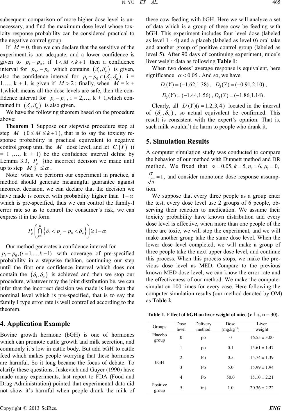

N. YU ET AL.
465
subsequent comparison of more higher dose level is un-
necessary, and find the maximum dose level whose tox-
icity response probability can be considered practical to
the negative control group.
If
M
= 0, then we can declare that the sensitive of the
experiment is not adequate, and a lower confidence is
given to
0k
pp−
; if
11Mk< <+
then a confidence
interval for 0M
pp
− which contains
( )
,
lu
δδ
is given,
also the confidence interval for
( )
0
,
i lu
pp δδ −∈
, i =
1,…, k + 1, is given if
2M>
; finally, when
M
= k +
1,which means all the dose levels are safe, then the con-
fidence interval for
0i
pp−
, i = 2,…, k + 1,which con-
tained in
( )
,
lu
δδ
is also given.
We have the following theorem based on the procedure
above:
Theorem 1 Suppose our stepwise procedure stop at
step
M
(
01Mk≤ ≤+
), that is to say the toxicity re-
sponse probability is practical equivalent to negative
control group until the
M
dose level, and let
( )
i
CY
(i
= 1 ,…, k + 1) be the confidence interval define by
Lemma 3.3,
p
P
{the incorrect decision we made until
up to step
M
}
α ≤
.
Note: when we perform our experiment in practice, a
method should generate meaningful guarantee against
incorrect decision, we can declare that the decision we
have made is correct with probability higher than
1 α −
which is pre-specified, thus we can control the family-I
error rate so as to control the consumer’s risk, we can
express it in the form
{ }
0
1
1
M
p lju
j
P pp δ δα
=

< − <≥−



Our method generates a confidence interval for
0
,( 1,...,1)
i
p pik−= +
with coverage of pre-specified
probability in a stepwise fashion, continuing our step
until the first one confidence interval which does not
contain the
( )
,
lu
δδ
is achieved and then we stop our
procedure, whatever may the joint distribution be, we can
infer that the incorrect decision we made is less than the
nominal level which is pre-specified, that is to say the
family I type error rate is well controlled accord ing to the
theorem.
4. Application Example
Bovine growth hormone (bGH) is one of hormones
which can promote cattle growth and milk secretion, and
commonly it’s low in cattle body. But add bGH to cattle
feed which makes people worrying that these hormones
are harmful. So it long became the focus of debate. To
clarify these questions, Juskevich and Guyer (1990) have
made many experiments, last report to FDA (Food and
Drug Administration) pointed that experimental data did
not show it’s harmful when people drank the milk of
these cow feeding with bGH. Here we will analyze a set
of data which is a group of these cow be feeding with
bGH. This experiment includes four level dose (labeled
as level 1 - 4) and a placeb (labeled as level 0) oral take
and another group of positive control group (labeled as
level 5). After 90 days of continuing experiment, mice’s
liver weight data as following Table 1:
When two doses’ average response is equivalent, here
significance
0.05 α <
. And so, we have
1()( 1.62,1.38)DY= −,
2
()( 0.91,2.10)DY= −
,
3()( 1.44,1.56)DY= −
,
4()( 1.86,1.14)DY= −
.
Clearly, all
( )(1,2,3,4)
i
DY i=
located in the interval
of
(, )
LU
δδ , so actual equivalent be confirmed. This
result is consistent with the expert’s opinion. That is,
such milk wouldn’t do harm to people who drank it.
5. Simulation Results
A computer simulation study was conducted to compare
the behavior of our method with Dunnett method and DR
method. We fixed that 1 0.05, 5,6,0,
i
kn αµ
====
1
n
σ
=
, and consider monotone dose response assump-
tion.
We suppose that every three people as a group enter
the test, every dose level use 2 groups of 6 people, ob-
serving their reaction to medication. We assume their
toxicity probability have known distribution and every
dose level is effective, when more than on e people of the
three are toxic, we will stop the experiment, and we will
make another group take the same dose level. When the
lower dose level completed, we will make a group of
three people take the next upper dose level, and continue
this process. When this process stops, we make the pre-
vious dose level as MED. Compare to the previous
known MED dose level, we can know the error rate and
the effectiveness of our method. We make the computer
simulation 100 times for every case. Here following the
computer simulation results (our method denoted by OM)
as Table 2.
Table 1. Effect of bGH on liver weight of mice (x
±
s, n = 30).
Groups
Dose
level
Delivery
method
Dose
(mg.kg−1)
Liver
weight
Placebo
group
0 po 0 16.55 ± 3.00
bGH
1 po 0.1 15.61 ± 1.47
2 Po 0.5 15.74 ± 1.39
3 Po 5.0 15.99 ± 1.94
4 Po 50.0 15.10 ± 2.21
Positive
group 5 inj 1.0 20.36 ± 2.22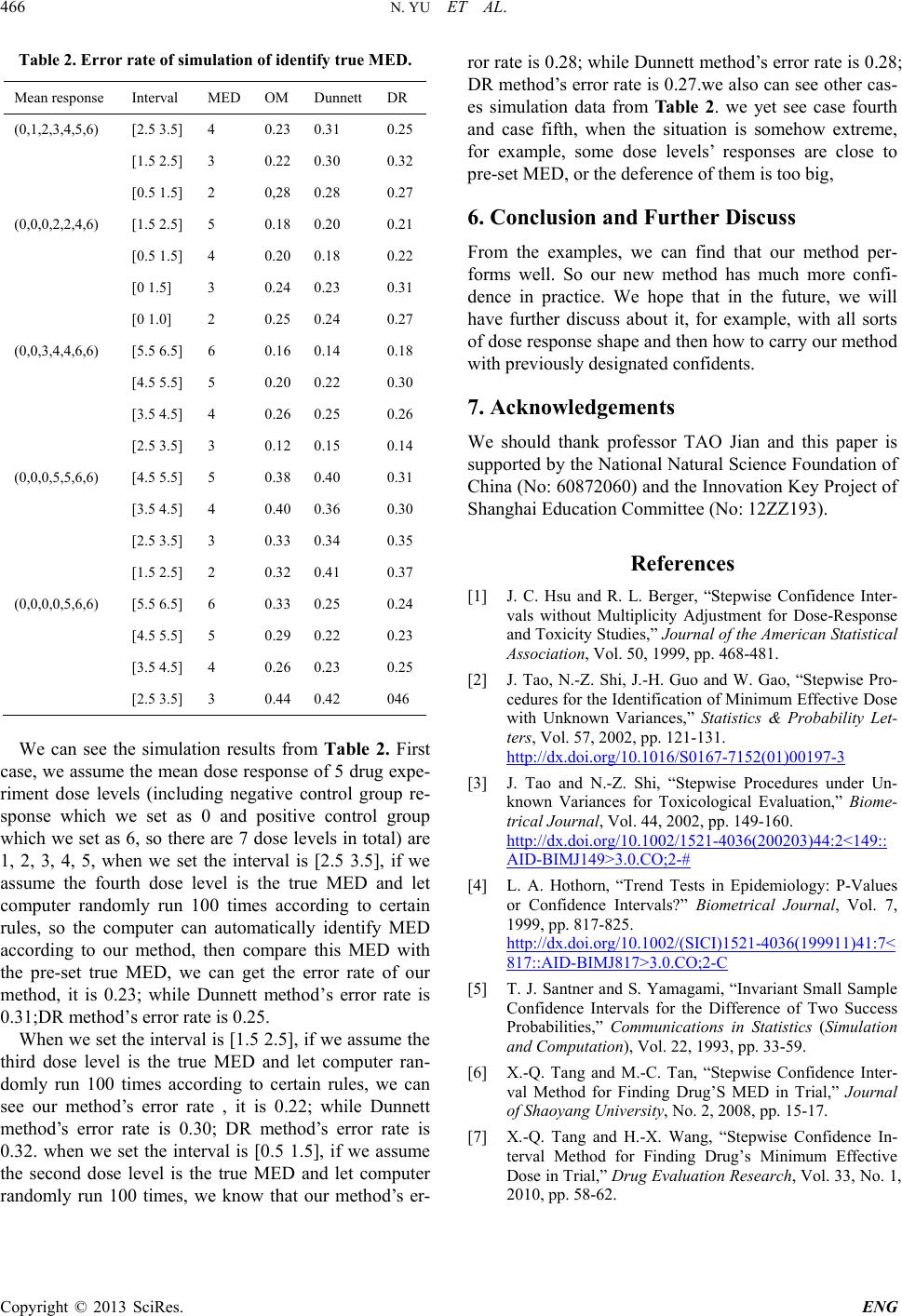

N. YU ET AL.
466
Table 2. Error rate of simulation of identify true MED.
Mean response Interval MED OM Dunnett DR
(0,1,2,3,4,5,6) [2.5 3.5] 4 0.23 0.31 0.25
[1.5 2.5] 3 0.22 0.30 0.32
[0.5 1.5] 2 0,28 0.28 0.27
(0,0,0,2,2,4,6) [1.5 2.5] 5 0.18 0.20 0.21
[0.5 1.5] 4 0.20 0.18 0.22
[0 1.5] 3 0.24 0.23 0.31
[0 1.0] 2 0.25 0.24 0.27
(0,0,3,4,4,6,6) [5.5 6.5] 6 0.16 0.14 0.18
[4.5 5.5] 5 0.20 0.22 0.30
[3.5 4.5] 4 0.26 0.25 0.26
[2.5 3.5] 3 0.12 0.15 0.14
(0,0,0,5,5,6,6) [4.5 5.5] 5 0.38 0.40 0.31
[3.5 4.5] 4 0.40 0.36 0.30
[2.5 3.5] 3 0.33 0.34 0.35
[1.5 2.5] 2 0.32 0.41 0.37
(0,0,0,0,5,6,6) [5.5 6.5] 6 0.33 0.25 0.24
[4.5 5.5] 5 0.29 0.22 0.23
[3.5 4.5] 4 0.26 0.23 0.25
[2.5 3.5] 3 0.44 0.42 046
We can see the simulation results from Table 2. First
case, we assume the mean dose response of 5 drug expe-
riment dose levels (including negative control group re-
sponse which we set as 0 and positive control group
which we set as 6, so there are 7 dose levels in total) are
1, 2, 3, 4, 5, when we set the interval is [2.5 3.5], if we
assume the fourth dose level is the true MED and let
computer randomly run 100 times according to certain
rules, so the computer can automatically identify MED
according to our method, then compare this MED with
the pre-set true MED, we can get the error rate of our
method, it is 0.23; while Dunnett method’s error rate is
0.31;DR method’s error rate is 0.25.
When we set the interval is [1.5 2.5], if we assume the
third dose level is the true MED and let computer ran-
domly run 100 times according to certain rules, we can
see our method’s error rate , it is 0.22; while Dunnett
method’s error rate is 0.30; DR method’s error rate is
0.32. when we set the interval is [0.5 1.5], if we assume
the second dose level is the true MED and let computer
randomly run 100 times, we know that our method’s er-
ror rate is 0.28; while Du nnett method’s error rate is 0.28;
DR method’s error rate is 0.27.we also can see other cas-
es simulation data from Ta b le 2 . we yet see case fourth
and case fifth, when the situation is somehow extreme,
for example, some dose levels’ responses are close to
pre-set MED, or the deference of them is too big,
6. Conclusion and Further Discuss
From the examples, we can find that our method per-
forms well. So our new method has much more confi-
dence in practice. We hope that in the future, we will
have further discuss about it, for example, with all sorts
of dose response shap e and then how to carry our method
with previously designated confidents.
7. Acknowledgements
We should thank professor TAO Jian and this paper is
supported by the National Natural Science Foundation of
China (No: 60872060) and the Innov ation Key Projec t of
Shanghai Education Committee (No: 12ZZ193).
References
[1] J. C. Hsu and R. L. Berger, “Stepwise Confidence Inter-
vals without Multiplicity Adjustment for Dose-Response
and Toxicity Studies,” J ournal of the American Statistical
Association, Vol. 50, 1999, pp. 468-481.
[2] J. Tao, N.-Z. Shi, J.-H. Guo and W. Gao, “Stepwise Pro-
cedures for the Identification of Minimum Effective Dose
with Unknown Variances,” Statistics & Probability Let-
ters, Vol. 57, 2002, pp. 121-131.
http://dx.doi.org/10.1016/S0167-7152(01)00197-3
[3] J. Tao and N.-Z. Shi, “Stepwise Procedures under Un-
known Variances for Toxicological Evaluation,” Biom e-
trical Journal, Vol . 44, 2002, pp. 149-160.
http://dx.doi.org/10.1002/1521-4036(200203)44:2<149::
AID-BIMJ149>3.0.CO;2-#
[4] L. A. Hothorn, “Trend Tests in Epidemiology: P-Values
or Confidence Intervals?” Biometrical Journal, Vol. 7,
1999, pp. 817-825.
http://dx.doi.org/10.1002/(SICI)1521-4036(199911)41:7<
817::AID-BIMJ817>3.0.CO;2-C
[5] T. J. Santner and S. Yamagami, “Invariant Small Sample
Confidence Intervals for the Difference of Two Success
Probabilities,” Communications in Statistics (Simulation
and Computation), Vol. 22, 1993, pp. 33-59.
[6] X.-Q. Tang and M.-C. Tan, “Stepwise Confidence Inter-
val Method for Finding Drug’S MED in Trial,” Journal
of Shaoyang University, No. 2, 2008, pp. 15-17.
[7] X.-Q. Tang and H.-X. Wang, “Stepwise Confidence In-
terval Method for Finding Drug’s Minimum Effective
Dose in Trial,” Drug Evaluation Research, Vol. 33, No. 1,
2010, pp. 58-62.