 Open Journal of Social Sciences 2013. Vol.1, No.7, 6-11 Published Online December 2013 in SciRes (http://www.scirp.org/journal/jss) http://dx.doi.org/10.4236/jss.2013.17002 Open Access A Collaborative Business Model for Imperfect Process with Setup Cost and Lead Time Reductions Chien-Chung Lo Department of Business Management, National United University, Miaoli, Chinese Taipei Email: low@ nuu.edu.tw Received October 2013 This paper develops a collaborative business model for imperfect process with setup cost and lead time reductions. We propose a simple solution procedure to derive the optimal order quantity, lead time, deli- very frequency and setup cost. Shortage during the lead time is assumed to be partially backordered. Nu- merical examples are carried out to show how the proposed model can result in a substantial cost savings over the traditional model. Keywords: Collaborative Model; Imperfect Process; Lead Time Reduction; Setup Cost Reduction Introduction Strategic business alliance is a formalized type of collabora- tive relationship between a vendor and a buyer in a supply chain. It involves commitment to long-term cooperation, shared benefits, joint problem solving and information sharing. This close partnership will ultimately improve product quality and reduce inventory cost and lead time of the supply chain. (Goya l, 1976) was one of the first authors to develop an in- tegrated inventory model for a single supplier-single customer problem. The joint vendor-buyer optimization was later rein- forced by (Banerjee, 1986; Goyal , 1988). (Lu, 1995; Hill 1997) presented a cooperative multiple deliveries policy. (Ha & Kim, 2003) considered a simple JIT single-setup multi-delivery mo- del and a single-setup single-delivery (SSSD) model. (Yang & Wee, 2000) considered an integration issue in an integrated deteriorating model. However, the quality related issues and the benefits of the setup cost and lead time reduction were not ad- dressed in these integrated models. Setup cost reduction is one of the important production ac- tivities in an integrated inventory control. In practice, setup cost can be reduced through worker training, procedural changes and specialized equipment acquisition. (Porteus, 1986) studied the impact of investing in reducing setup cost by considering the discounted model. (Affisco, Paknejad, & Nasri, 1988, 2002) addressed the joint optimization cost of the vendor and the buye r. They showe d tha t by investing in setup cost reduction of the vendor, a significant saving in joint total cost can be achieved. (Nasri, Paknejad, & Affisco, 1991) extended Baner- jee’s model to investigate the impact of investing in setup cost and ordering cost reductions simultaneously. Their results indi- cated that both the vendor and the buyer can realize significant savings. Lead time reduction is another important production activity in an integrated inventory control. Lead time consists of order preparation, order transmittal, order processing and assembly, additional stock acquisition time and delivery time (Ballou, 2004). In most cases, lead time can be shortened with an added crashing cost. Recently, (Ouyang, Yeh, & Wu, 1996) extended the (Q, r) model by (Ben -Daya & Raouf, 1994) to consider the lead time effect and incorporate the partial backordering into the inventory model. (Hari ga , 1999) studied the relationship between lot size and lead time in the process time aspect. (Pan & Yang, 2002) p resented an integ rated supplier-purchaser model with controllable lead time. The model has a substantial cost saving when lead time is controll able. (Chen, Chang, & Ouyang, 2001) presented a continuous review inventory model when ordering cost is dependent on lead time. (Ben-Daya & H a riga, 2003) developed a continuous review inventory model where lead time is considered as a controllable variable. Lead time is decomposed into all its components: set-uptime, processing time and non-productive time. Later, (O uyang, Wu, & Ho, 2004) extended Pan and Yang’s model by allowing shortages. In a real system, due to the imperfect production process of the vendor and the damages during the transportation process from the vendor to the buyer, goods re ceived by the buyer may contain some percentage of defectives. Recently, (Salameh & Jaber, 2000) examined a joint EOQ lot sizing and inspection policy with imperfect quality. They assumed 100% screening and all poor-quality items were sold at the end of the screening process. (Goyal, Huang, & Chen, 2003; Hua ng, 2004) extended Salameh and Jaber’s model and proposed an integrated ven- dor-buyer cooperative inventory model for items with imperfect quality. (Parachristos & Konstantaras, 2006) pointed out some drawback in Salameh and Jaber’s model regarding ensuring no shortage occurrence. They extended the model by Salameh and Jaber to consider withdraw at the end of the planning horizon, and consider different inspection process with Bernoulli ran- dom vari able and suffic ient conditio n to prevent shor tage. (Chung & Huang 2006) modified two assumptions of the classical EOQ model to reflect the real-life situations. Their study incorpo- rated the model by (Salameh & Jaber, 2000) to consider a re- tailer’s production/inventory model with imperfect quality and permissible delay in payments. In our integrated business model, lead time demand is consi- dered to be normally distributed. We derive the joint total ex- pected cost function for the partners and propose a simple algo- rithm procedure to derive the optimal integrated business model policy. Finally, numerical examples are carried out to show how the proposed model can result in a substantial cost savings  C.-C. LO Open Access over the traditional model. Notation and Assumptions The notation used in our model is shown as follows: D: average demand per year for the buyer P: production rate of the vendor A: per ordering cost for the buyer A0: original ordering cost S: per setup cost for the vendor (decision variable) S0: original setup cost I(S): capital investment in reducing the vendor’s setup cost; ( ) 00 ()ln/,for 0 S ISCS SSS= <≤ , where the parameter CS = 1/θ and θ denotes the percentage decrease in S per dollar increase in I(S) αS: the fractional cost of the vendor’s capital investment Cb: unit purchase cost paid by the buyer Cv: unit production cost paid by the vendor rb: inventory carrying cost percentage per year per dollar for the buyer rv: inventory carrying cost percentage per year per dollar for the vendor π: stock-out cost per unit short for the buyer π0: marginal profit per unit for the buyer β: fraction of the shortage that will be backordered, γ: screening rate for the buyer t: screening period for each arrival lot u: screening cost per unit for the buyer v: warranty cost of defective items per unit for the vendor R: reorder point of the buyer (decision variable) Q: order quantity of the buyer (decision variable) L: length of lead time for the buyer (decision variable) L0: original length of lead time m: number of lots in which the items are delivered from the vendor to the buyer in one production cycle (decision variable) X: lead time demand which has a cumulative distribution function (c.d.f.) F with finite mean DL and standard deviation , where denotes the standard deviation of demand per unit time. Y: percentage of defective items in Q f(y): probability density function of Y : standard normal probability density function : standard normal cumulative distribution function : expected value TCb: total expected annual cost for the buyer TCv: total expected annual cost for the vendor JTC: joint total expected cost including TCb and TCv It is assumed that the buyer adopts a continuous review in- ventory policy where lead time can be reduced by a crashing cost. The vendor may also invest in setup cost reduction. The imperfect production process of the vendor results in random defective items. As a result, an order received by the buyer has a certain percentage of defective items. Since 100% screening process is used, all the defective items are screened out and discarded. Other assumptions for our model are: • R = DL + k , where SS = k and k is the safety factor. • Shortages are partially backordered. • The lead time L has n mutually independent components. The ith component has a minimum duration ai and normal dura- tion bi, and a crashing cost ci per unit time. The components can be rearranged such that . The components are crashed from the least crashing cost per unit time. • The lead time and ordering cost reductions have the fol- lowing relationship: where τ (<0) is constant scaling parameter for the logarithmic relationship between percentages in lead time reductions and ordering cost. • Y and the buyer’s demand are independent random vari- ables. • The extra costs incurred by the vendor will be fully trans- ferred to the buyer if shortened lead time is requested. • The number of good units is equal or greater than the de- mand during the screening period. Model Formulation The shortage quantity at the end of the buyer’s replenishment cycle i s (X − R)+ and the order cycle length of the buyer is (1 − Y)Q/D, where X and Y are assumed to be independent random variables. Hence, the expected annual stock-out cost for the buyer is. ( )( ) ( ) ()() 0 0 11 11 1 DX R EYQ D EEX R YQ ππ β ππ β + + − +− − =+− − − (1) The net inventory level of the good items at the epoch before and after receipt of an order is R − DL + (1 − β)E(X − R)+ and [1 − E(Y)]Q + R − DL + (1 − β)E(X − R)+ respectively. The average inventory of good items is [1 − E(Y)]Q/2 + R − DL + (1 − β)E(X − R)+. Since the defective items are discarded after the screening process, the buyer’s expected defective item inven- tory is E{tQY/[(1 − Y)Q/D]} = E[Y/(1 −Y)]QD/γ. The total ex- pected inventory carrying cost per year for the buyer is ( ) ()( ) 1 12 (1 ) bb EY Q Y QD E rC Y RDLE XR γ β + − + − + −+−− (2) Let Li be the length of lead time with components crashed to their minimum duration, then Li can be expressed as ( ) ( ) 01 11 ,1, 2,..., i i jj j ni j jj jj LL ba bbain = = = =−− =−− = ∑ ∑∑ (3) The lead time crashing cost C(L) per cycle for a given [Li, L i−1] is ( )() ( ) 1 11 i iijj j j CLc LLcba − − = = −+− ∑ (4) Therefore, the expected lead time crashing cost per year for the buyer is E{C(L)/[(1 − Y)Q/D]} = E[1/(1 − Y)]DC(L)/Q. From assumption (4), the lead time L and ordering cost A have a relationship: (5) Equation (5) can be rewritten as 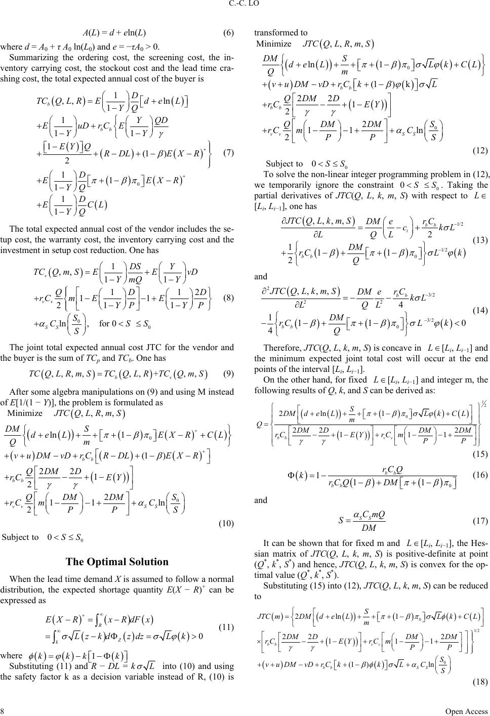 C.-C. LO Open Access A(L) = d + eln(L) (6) where d = A0 + τ A0 ln(L0) and e = −τA0 > 0. Summarizing the ordering cost, the screening cost, the in- ventory carrying cost, the stockout cost and the lead time cra- shing cost, the total expected annual cost of the buyer is ()( ) ( )()( ) ( )() ( ) 0 1 , ,ln 1 1 11 1(1 ) 2 11 11 1 b bb D TCQ L REdeL YQ Y QD EuDr CE YY EY QRDLE XR D EEX R YQ D E CL YQ γ β π βπ + + =+ − ++ −− − ++ −+−− ++ −− − + − (7) The total expected annual cost of the vendor includes the se- tup cost, the warranty cost, the inventory carrying cost and the investment in setup cost reduction. One has ( ) 00 1 ,, 11 1 12 11 21 1 ln,for0 v vv SS DS Y TC QmSEEvD Y mQY QDD rCm EE YPY P S C SS S α = + −− + −−+ −− + <≤ (8) The joint total expected annual cost JTC for the vendor and the buyer is the sum of TCp and TCb. One has ()() () ,,,,,,+,, bv TC Q L R mSTCQ L RTCQm S= (9) After some algebra manipulations on (9) and using M instead of E[1/(1 − Y)], the problem is formulated as ( ) Minimize, ,,,JTCQLR m S ( ) ( ) ()()( ) ( )()() ( ) ( ) 0 0 ln 1 (1 ) 22 1 2 2 1 1ln 2 bb bb vvS S DM S d eLEXRCL Qm vuDMvDr CRDLEXR Q DMD rCE Y Q DMDMS rC mC PP S π βπ β γγ α + + +++ +−−+ ++−+−+−− +−+− +− −++ (10) The Optimal Solution When the lead time demand X is assumed to follow a normal distribution, the expected shortage quantity E(X − R)+ can be expressed as ()()( ) ()( )( ) 0 R Z k EXRxR dFx Lzk dzdzLk σ σϕ ∞ + ∞ −= − =−Φ => ∫ ∫ (11) where ( )( )( ) 1k kkk φϕ =− −Φ Substituting (11) and R − DL = k into (10) and using the safety factor k as a decision variable instead of R, (10) is transformed to ( ) Minimize, ,,,JTCQLR m S ( ) ( ) ()( )() ()( ) ( ) ( ) 0 0 ln 1 (1) k 22 1 2 2 1 1ln 2 bb bb vvS S DM S d eLLkCL Qm vuDMvDr CkL Q DMD rCE Y Q DMDMS rC mC PP S πβπ σϕ βϕ σ γγ α +++ +−+ ++−++ − +− +− +−−++ (12) To solve the non-linear integer programming problem in (12), we temporarily ignore the constraint . Taking the partial derivatives of JTC(Q, L, k, m, S) with respect to [Li, Li−1], one has ( ) ( )( )() 1/2 1/2 0 ,,, , 2 111 2 bb i bb JTC QLkmSDMerC c kL L QL DM rCL k Q σ βπβπ σϕ − − ∂ = −+ ∂ +−++ − (13) and ( ) ( )()( ) 23/2 22 3/2 0 ,,, , 4 111 0 4 bb bb JTC QLkmSDMer CkL L QL DM rCL k Q σ βπβπ σϕ − − ∂=−− ∂ −−++ −< (14) Therefore, JTC(Q, L, k, m, S) is concave in [Li, Li−1] and the minimum expected joint total cost will occur at the end points of the interval [Li, Li−1]. On the other hand, for fixed [Li, Li−1] and integer m, the following results of Q, k, and S can be derived as: ( ) ( ) ( )( )() ( ) ( ) 12 0 2 ln1 22 2 1 11 bb vv S DMdeLLkCL m QDM DDMDM rCE YrCmPP πβπσϕ γγ ++++−+ = −+ −+−−+ (15) ( )( )( ) 0 111 bb bb rCQ kr CQDM βπ βπ Φ=− −++ − (16) and (17) It can be shown that for fixed m and [Li, Li−1], the Hes- sian matrix of JTC(Q, L, k, m, S) is positive-definite at point (Q*, k*, S*) and hence, JTC(Q, L, k, m, S) is convex for the op- timal value (Q*, k*, S*). Substituting (15) into (12), JTC(Q, L, k, m, S) can be reduced to ()( ) ( ) ()( )() ( ) ( ) ()( ) 0 1/2 0 2 ln1 22 2 1 11 (1 )ln bb vv bbS S S JTC mDMdeLLkC L m DM DDMDM rCEYrCmPP S vuDMvDr CkkLCS πβπ σφ γγ βφ σα =+++ +−+ ×−+ −+−−+ ++−++− + (18) 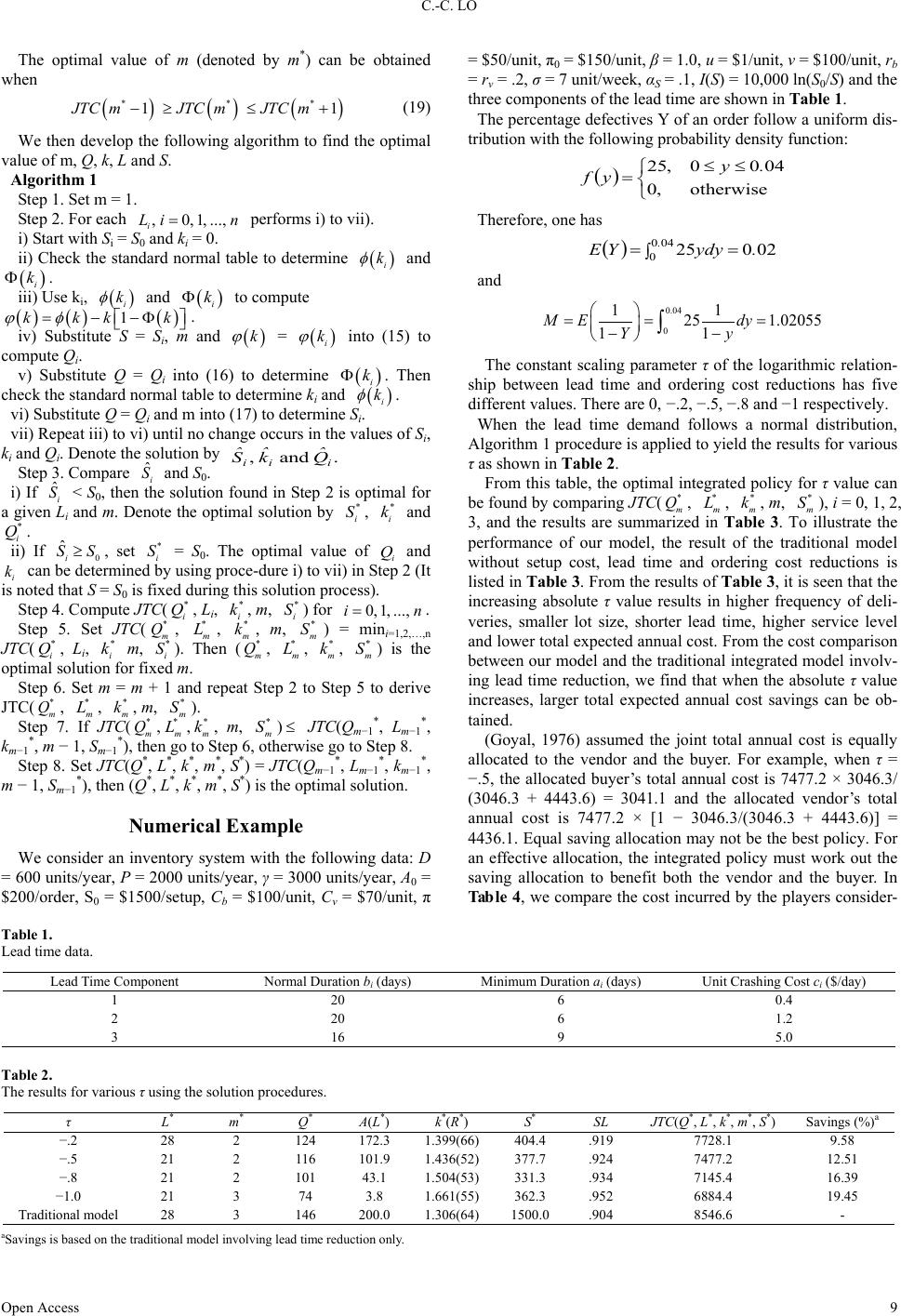 C.-C. LO Open Access The optimal value of m (denoted by m*) can be obtained when () () () * ** 11JTC mJTC mJTC m−≥≤ + (19) We then develop the following algorithm to find the optimal value of m, Q, k, L and S. Algorithm 1 Step 1. Set m = 1. Step 2. For each performs i) to vii). i) Start with Si = S0 and ki = 0. ii) Check the standard normal table to determine and . iii) Use ki, and to compute ( )( )() 1k kkk ϕφ =− −Φ . iv) Substitute S = Si, m and = into (15) to compute Qi. v) Substitute Q = Qi into (16) to determine . Then check the standard normal table to determine ki and . vi) Substitute Q = Qi and m into (17) to determine Si. vii) Repeat iii) to vi) until no change occurs in the values of Si, ki and Qi. Denote the solution by Step 3. Compare and S0. i) If < S0, then the solution found in Step 2 is optimal for a give n Li and m. Denote the optimal solution by , and . ii) If , set = S0. The optimal value of and can be determined by using proce-dure i) to vii) in Step 2 (It is noted that S = S0 is fixed during this solution process). Step 4. Compute JTC( , Li, , m, ) for . Step 5. Set JTC( , , , m, ) = mini=1,2,…,n JTC( , Li, m, ). Then ( , , , ) is the optimal solution for fixed m. Step 6. Set m = m + 1 and repeat Step 2 to Step 5 to derive JTC( , , , m, ). Step 7. If JTC( , , , m, ) JTC(Qm−1*, Lm−1*, km−1*, m − 1, Sm−1*), then go to Step 6, otherwise go to Step 8. Step 8. Set JTC(Q*, L*, k*, m*, S*) = JTC(Qm−1*, Lm−1*, km−1*, m − 1, Sm−1*), then (Q*, L*, k*, m*, S*) is the optimal solution. Numerical Example We consider an inventory system with the following data: D = 600 units/year, P = 2000 units/year, γ = 3000 units/year, A0 = $200/order, S0 = $1500/setup, Cb = $100/unit, Cv = $70/unit, π = $50/unit, π0 = $150/unit, β = 1.0, u = $1/unit, v = $100/unit, rb = rv = .2, σ = 7 unit/week, αS = .1, I(S) = 10,000 ln(S0/S) and the three components of the lead time are shown in Table 1. The percentage defectives Y of an order follow a uniform dis- tribution with the following probability density function: ( ) ≤≤ =otherwise,0 0400,25 .y yf Therefore, one has and 0.04 0 11 25 1.02055 11 M Edy = == −− ∫ The constant scaling parameter τ of the logarithmic relation- ship between lead time and ordering cost reductions has five different values. There are 0, −.2, −.5, −.8 and −1 respectively. When the lead time demand follows a normal distribution, Algorithm 1 procedure is applied to yield the results for various τ as shown in Table 2. From this table, the optimal integrated policy for τ value can be found by comparing JTC( , , , m, ), i = 0, 1, 2, 3, and the results are summarized in Table 3. To illustrate the performance of our model, the result of the traditional model without setup cost, lead time and ordering cost reductions is listed in Table 3. From the results of Table 3, it is s een tha t the increasing absolute τ value results in higher frequency of deli- veries, smaller lot size, shorter lead time, higher service level and lower total expected annual cost. From the cost comparison between our model and the traditional integrated model involv- ing lead time reduction, we find that when the absolute τ value increases, larger total expected annual cost savings can be ob- tained. (Goyal, 1976) assumed the joint total annual cost is equally allocated to the vendor and the buyer. For example, when τ = −.5, the allocated buyer ’s total annual cost is 7477.2 × 3046.3/ (3046.3 + 4443.6) = 3041.1 and the allocated vendor’s total annual cost is 7477.2 × [1 − 3046.3/(3046.3 + 4443.6)] = 4436.1. Equal saving allocation may not be the best policy. For an effective allocation, the integrated policy must work out the saving allocation to benefit both the vendor and the buyer. In Table 4, we compare the cost incurred by the players consider- Table 1. Lead time data. Lead Time Component Normal Duration bi (days) Minimum Duration ai (days) Unit Crashing Cost ci ($/day) 1 20 6 0.4 2 20 6 1.2 3 16 9 5.0 Table 2. The results for various τ using the solution procedures. τ L m Q A(L ) k (R ) S SL JTC(Q , L , k , m , S ) Savings (% ) −.2 28 2 124 172.3 1.399(66) 404.4 .919 7728.1 9.58 −.5 21 2 116 101.9 1.436(52) 377.7 .924 7477.2 12.51 −.8 21 2 101 43.1 1.504(53) 331.3 .934 7145.4 16.39 −1.0 21 3 74 3.8 1.661(55) 362.3 .952 6884.4 19.45 Traditional model 28 3 146 200.0 1.306(64) 1500.0 .904 8546.6 - aSavings is ba sed o n the tr ad iti on al m ode l i nvo lv i ng lea d time reduction on ly. 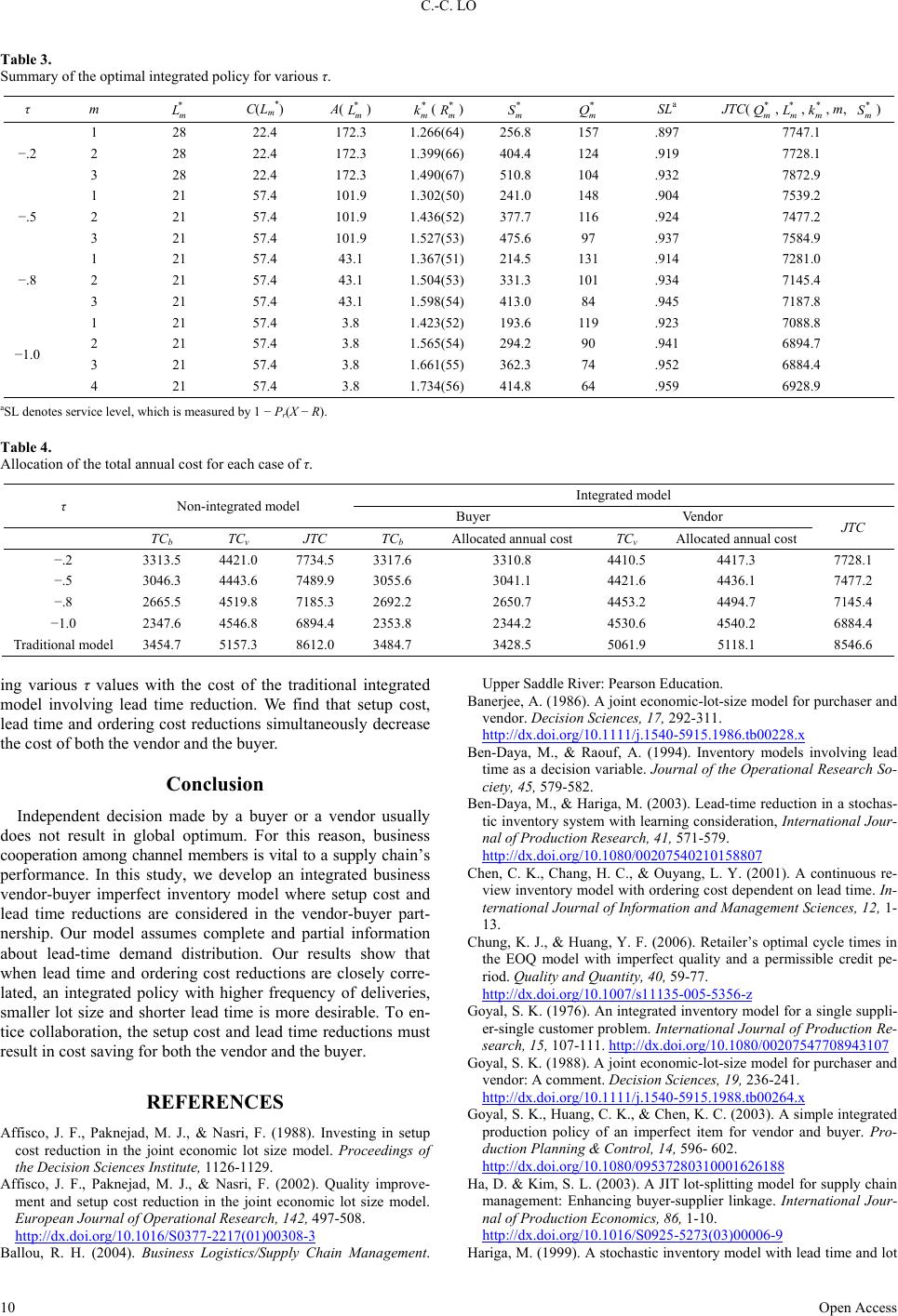 C.-C. LO Open Access Table 3. Summary of the optimal integrated policy for various τ. τ m C(Lm*) A( ) ( ) SLa JTC( , , , m, ) −.2 1 28 22.4 172.3 1.266(64) 256.8 157 .897 7747.1 2 28 22.4 172.3 1.399(66) 404.4 124 .919 7728.1 3 28 22.4 172.3 1.490(67) 510.8 104 .932 7872.9 −.5 1 21 57.4 101.9 1.302(50) 241.0 148 .904 7539.2 2 21 57.4 101.9 1.436(52) 377.7 11 6 .924 7477.2 3 21 57.4 101.9 1.527(53) 475.6 97 .937 7584.9 −.8 1 21 57.4 43.1 1.367(51) 214.5 131 .914 7281.0 2 21 57.4 43.1 1.504(53) 331.3 101 .934 7145.4 3 21 57.4 43.1 1.598(54) 413.0 84 .945 7187.8 −1.0 1 21 57.4 3.8 1.423(52) 193.6 11 9 .923 7088.8 2 21 57.4 3.8 1.565(54) 294.2 90 .941 6894.7 3 21 57.4 3.8 1.661(55) 362.3 74 .952 6884.4 4 21 57.4 3.8 1.734(56) 414.8 64 .959 6928.9 aSL denotes service level, which is measured by 1 − Pr(X − R). Table 4. Allocation of the total annual cost for each case of τ. τ Non-integrated model Integrated model Buyer Vendor JTC TCb TCv JTC TCb Allocated annual cos t TCv Allocated annual cost −.2 3313.5 4421.0 7734.5 3317.6 3310.8 4410.5 4417.3 7728.1 −.5 3046.3 4443.6 7489.9 3055.6 3041.1 4421.6 4436.1 7477.2 −.8 2665.5 4519.8 7185.3 2692.2 2650.7 4453.2 4494.7 7145.4 −1.0 2347.6 4546.8 6894.4 2353.8 2344.2 4530.6 4540.2 6884.4 Traditional model 3454.7 5157.3 8612.0 3484.7 3428.5 5061.9 5118.1 8546.6 ing various τ values with the cost of the traditional integrated model involving lead time reduction. We find that setup cost, lead time and ordering cost reductions simultaneously decrease the cost of both the vendor and the buyer. Conclusion Independent decision made by a buyer or a vendor usually does not result in global optimum. For this reason, business cooperation among channel me mbers is vital to a supply chain’s performance. In this study, we develop an integrated business vendor-buyer imperfect inventory model where setup cost and lead time reductions are considered in the vendor-buyer part- nership. Our model assumes complete and partial information about lead-time demand distribution. Our results show that when lead time and ordering cost reductions are closely corre- lated, an integrated policy with higher frequency of deliveries, smaller lot size and shorter lead time is more desirable. To en- tice collaboration, the setup cost and lead time reductions must result in cost saving for both the vendor and the buyer. REFERENCES Affisco, J. F., Paknejad, M. J., & Nasri, F. (1988). Investing in setup cost reduction in the joint economic lot size model. Proceedings of the Decision Sciences Institute, 1126-1129. Affisco, J. F., Paknejad, M. J., & Nasri, F. (2002). Quality improve- ment and setup cost reduction in the joint economic lot size model. European Journal of Operational Research, 142, 497-508. http://dx.doi.org/10.1016/S0377-2217(01)00308-3 Ballou, R. H. (2004). Business Logistics/Supply Chain Management. Upper Saddle River: Pearson Education. Banerjee, A. (1986). A joint econo mic-lot-size model for p urchaser and vendor. Decision Sciences, 17, 292-311. http://dx.doi.org/10.1111/j.1540-5915.1986.tb00228.x Ben-Daya, M., & Raouf, A. (1994). Inventory models involving lead time as a decision v ariable. Journal of the Operational Research So- ciety, 45, 579-582. Ben-Daya, M., & Harig a, M. (2003). Lead-time reducti on in a stochas- tic inventory system with learning consideration, International Jour- nal of Production Research, 41, 571-579. http://dx.doi.org/10.1080/00207540210158807 Chen, C. K., Chang, H. C., & Ouyang, L. Y. (2001). A continuous re- view inventory model with ordering cost dependent on lead time. In- ternational Journal of Information and Management Sciences, 12, 1- 13. Chung, K. J., & Huang, Y. F. (2006). Retailer’s optimal cycle times in the EOQ model with imperfect quality and a permissible credit pe- riod. Quality and Quantity, 40, 59-77. http://dx.doi.org/10.1007/s11135-005-5356-z Goyal, S. K. (1976). An integrated inventory model for a s ingle suppli- er-single customer prob lem. International Journal of Production Re- search, 15, 107-111. http://dx.doi.org/10.1080/00207547708943107 Goyal, S. K. (1988). A joint econo mic-lot-size model for purchaser and vendor: A comment. Decision Sciences, 19, 236-241. http://dx.doi.org/10.1111/j.1540-5915.1988.tb00264.x Goyal, S. K., Huang , C. K., & Chen, K. C. (2003). A simple integ rated production policy of an imperfect item for vendor and buyer. Pro- duction Planning & Control, 14, 596- 602. http://dx.doi.org/10.1080/09537280310001626188 Ha, D. & Kim, S. L. (2003). A J IT lot-splitting model for supply chain management: Enhancing buyer-supplier linkage. International Jour- nal of Production Economics, 86, 1-10. http://dx.doi.org/10.1016/S0925-5273(03)00006-9 Hariga, M. (1999). A stochas tic inventory model with lead time and lot  C.-C. LO Open Access size interaction. Production Planning and Control, 10, 434-438. http://dx.doi.org/10.1080/095372899232957 Hill, R. M. (1997). The single-vendor single-buyer integrated produc- tion inventory model with a gen eralized policy. European Journal of Operational Research, 97, 493-499. http://dx.doi.org/10.1016/S0377-2217(96)00267-6 Huang, C. K. (2004). An optimal policy for a single-vendor single- buyer integrated pro duction-inventory problem with process unrelia- bility consideration. International Journal of Production Economics, 91, 91-98. http://dx.doi.org/10.1016/S0925-5273(03)00220-2 Lu, L. (1995). A one-vendor multi-buyer integrated inventory model. European Journal of Operational Research, 81, 312-323. http://dx.doi.org/10.1016/0377-2217(93)E0253-T Nasri, F., Paknejad, M. J., & Aff isco, J. F. (199 1). Si multaneous in vest- ment in setup cost and order cost reduction in the jo int economic lot size model. Proceedings of the Northeast Decision Sciences Institute, 263-267. Ouyang, L. Y., Yeh, N. C., & Wu, K. S. (1996). Mixture inventory mo- del with backorders and lost sales for variable lead time. Journal of the Operational Research Society, 47, 829-832. Ouyang, L. Y., Wu, K. S., & Ho, C. H. (2004). Integrated vendor-buyer cooperative model with stochastic demand in controllable lead time. International Journal of Production Economics, 92, 255-266. http://dx.doi.org/10.1016/j.ijpe.2003.10.016 Pan, J. C. H., & Yang, J. S. (2002). A study of an integrated inventory model with controllable lead time. International Journal of Produc- tion Research, 40, 1263-1273. http://dx.doi.org/10.1080/00207540110105680 Papachristos, S., & Konstan taras, I. (20 0 6). Econ o mic ordering q u antity models for items with imperfect quality. International Journal of Production Economics, 100, 148-154. http://dx.doi.org/10.1016/j.ijpe.2004.11.004 Porteus, E. L. (1986). Optimal lot sizing, process quality improvement and setup cost reduction. Operations Research, 34, 137-144. http://dx.doi.org/10.1287/opre.34.1.137 Salameh, M. K., & Jaber, M. Y. (2 000). Economic production quantity model for items wi th i mperfect qu ality. International Journal of Pro- duction Economics, 64, 59-64. http://dx.doi.org/10.1016/S0925-5273(99)00044-4 Yang, P. C. & Wee, H. M. (2000). Economic ordering policy of deteri- orated item for vendor and buyer: An integrated approach. Produc- tion Planning and Control, 11, 474-480. http://dx.doi.org/10.1080/09537280050051979
|