Interactions between House Prices, Stock Prices and Monetary Policy—Using Recursive VAR

doi:10.4236/ajibm.2013.38074

Paper Menu >>

Journal Menu >>

American Journal of Industrial and Business Management, 2013, 3, 645-654

Published Online December 2013 (http://www.scirp.org/journal/ajibm)

http://dx.doi.org/10.4236/ajibm.2013.38074

Open Access AJIBM

645

Interactions between House Prices, Stock Prices and

Monetary Policy—Using Recursive VAR

Chun-Chang Lee1, Chih-Min Liang2, Wen-Hui Wu1, Shu-Man You3

1Department of Real Estate Management, National Pingtung Institute of Commerce, Pingtung, Taiwan; 2Department of Public Fi-

nance and Tax Administration, National Taipei Institute of College of Business, Taipei, Taiwan; 3Department of Real Estate and

Built Environment, Natioanl Taipei University, New Taipei City, Taiwan.

Email: lcc@npic.edu.tw, ljimmy.ljimmy@msa.hinet.net, winnie0177@hotmail.com, youshuman@gmail.com

Received July 21st, 2013; revised August 21st, 2013; accepted August 29th, 2013

which permits unrestricted use, distribution, and reproduction in any medium, provided the original work is properly cited. In accor-

ABSTRACT

This paper uses a recursive VAR model to analyze the effects of monetary policy shock and the role of house price and

stock price shocks. The data come from the first quarter of 1993 to the second quarter of 2010 in Taiwan. There is em-

pirical evidence suggesting that house prices and stock prices do not play the role of a transmission mechanism for

monetary policy shocks. When house prices increase, stock prices undergo a simultaneous and significant increase, but

this effect gradually disappears. As house prices increase, the interest rate is simultaneously and positively affected; this

effect is insignificant until after the second quarter. As stock prices increase, house prices are positively affected, which

is consistent with the sign of the expected value, but the effect is insignificant. Under increasing stock prices, the inter-

est rate simultaneously increases, and this effect is significant during the third and tenth quarters.

Keywords: Asset; House Prices; Stock Prices; Monetary Policy; Recursive VAR

1. Introduction

The subprime crisis and a series of financial crises in the

US highlight the importance of asset prices as a trans-

mission mechanism for monetary policy changes. This

is primarily due to the central collateral role played by

asset prices such as house prices. Asset prices not only

affect the capital of financial institutions but also re-

sult in changes in overall corporate investment and

private consumption patterns, making these a source of

macroeconomic fluctuations. Bjørnland and Jacobsen

[1] suggested that central banks have managed to keep

inflation in check through inflation targeting, yet they

have not managed to prevent asset prices from burst-

ing and having real negative effects. A report by the

International Monetary Fund [2] noted that monetary

policy-makers should pay more attention to the overall

financial risk caused by the bursting of real property

bubbles. Due to the role played by the wealth storage of

assets, the impact of asset prices should be carefully

assessed in times of disturbance. Asset prices can

simultaneously respond to monetary policy and thus

become an important shock transmission mechanism

[3-5]. Hence, because of their timely response to

economic shocks, asset prices may be important

indicators of the status of monetary policy. An analysis

of the role played by asset prices as a transmission

mechanism of monetary policy can help to understand

whether monetary policy can effectively achieve its

goals.

Unlike other assets, houses have the dual role of being

a wealth storage mechanism as well as an important

durable consumption good. Changes in house prices can

affect the wealth of households. According to the Tobin

Q theory, when the value of a pledge rises, the rising

house price will stimulate housing construction activities .

House price shock may affect real output and commodity

price, making it an important forward-looking variable.

Hence, monetary policymakers will monitor house prices.

House prices can affect housing market development,

capital flows and prices in other markets. Past research

on the role house prices play in the overall economy has

often neglected the effect of other asset prices, leading to

Interactions between House Prices, Stock Prices and Monetary Policy—Using Recursive VAR

646

errors in the empirical results. Case et al. [6] noted that

the stock market and housing market have an important

effect on macroeconomic activity in a mature economy.

Hence, this study will also explore the role of stock price

shocks.

When estimating the relationships between macro-

economic variables, VAR (vector autoregression) analy-

sis, including three types of reduced form VAR, re-

cursive VAR, and SVAR (structural VAR), is often

applied. The reduced form VAR is a VAR model with-

out a priori limits that can perform an empirical study

without relying on any economic theory. Although it is

very convenient for analyzing the short-term dynamic re-

lationships between variables, the over-parameterization

of results in the VAR model reduce the estimation ef-

ficiency of the model, and the long-term relationships

between economic variables cannot be explained. Bernanke

and Blinder [7] noted that it is highly risky to use the

VAR model without limits in structural inference. Each

variable of the reduced form VAR model is a linear

function composed of the past value of the variable, the

past values of other variables, and errors, without con-

sidering the current impact in between variables. The

regression errors of the reduced form VAR are correlated

with the contemporaneous term, making it difficult to

identify the structural impact. Comparatively, there is no

correlation between the recursive VAR structural errors.

As IRF (impulse reaction function) requires no cor-

relation between shocks, the recursive VAR model is

also frequently used to illustrate the dynamic impact of

specific variables on the endogenous variables.

When using a recursive VAR model to measure the

structural effects caused by policy changes, the ordering

of monetary policy variables and other economic va-

riables should be conducted. The contemporaneous

impact between variables is of recursive form [8-9]. The

order of model endogenous variables is subject to the

contemporaneous relationship between monetary policy

and other economic variables. Compared with SVAR, the

identification of recursive VAR is simpler and more

straightforward.

This paper uses recursive VAR as the model setting

approach. Because monetary policy may affect asset

prices (stock and house prices) via the interest rate chan-

nel, this model illustrates the interactive relationship be-

tween asset price and monetary policy. When setting the

empirical model, this study also considers the potential

impact of asset prices on monetary policy to understand

the short-term interaction between monetary policy and

asset prices. The proposed model is a traditional closed

economy system model, which consists of macroeco-

nomic variables for monetary policy and asset prices to

explain the effect of changes in monetary policy and the

role of house and stock price shocks.

2. Empirical Model Setting

First, t is assumed to represent the stationary variable

vector in the macroeconomic respect :



51



ln, ln, ln, ln,

yGDPCPIHPSTOCKRATE



; the

endogenous variables in brackets represent output, con-

sumer price index, house prices, stock prices and interest

rate, respectively. If the VAR presentation equation of

y is









,







 

, and





L is an invertible matrix, then it can be written into

the equation of the moving average as follows:



yBL



 (1)

where t



is a







vector of reduced form residuals

assumed to be identically and independently distributed,





tiid





, with a positive definite covariance matrix







BL is the







convergent matrix polyno-

mial in the lag operator L,



BL BL





. Following

the literature, the innovations





are assumed to be

written as linear combinations of the underlying or-

thogonal structure disturbances





e, i.e., tt





. The

VAR can then be written in terms of structural shocks in

the following manner:





yBLSS CLe









(2)

where









CL BLS. If S is identified, we can derive

the MA representation in (2) as is calculated

from a reduced form estimation. To identify S, the et’s

are normalized so that they all have unit variance. The

normalization of







ecov t implies that SS





. Be-

cause the model contains five variables, the simultaneous

matrix S can identify as many as 15 parameters. There-

fore, the matrix S should be added with some restrictions

to identify structural disturbances.

With a five-variable VAR, we can identify five struc-

tural shocks, namely, the output shocks , the

consumer price index shocks , house price

shocks



ln GDP





ln CPI





e, stock price shocks



and

monetary policy shocks

ln STOCK





e. We then order the vector

of structural shocks as follows:

lnlnln ln

,,, ,

GDPCPIHPSTOCK MP

tttt tt

eee eee











This paper attempts to establish a recursive VAR

model and set constraints for the simultaneous variables,

ten of which are set to zero. No variable is assumed to be

affected by the variable that follows it in the contempo-

raneous term. Hence, in the recursive VAR model, dif-

ferences in the ordering of variables will affect the em-

Open Access AJIBM

Interactions between House Prices, Stock Prices and Monetary Policy—Using Recursive VAR 647

pirical results as well as the degree of response to shocks.

The variables in the model are ordered as follows: gross

domestic product and consumer price index are the proxy

macroeconomic variables; asset price is represented by

the Sinyi house price index and the weighted average of

the stock prices; finally, the weighted average lending

interest rate is the proxy variable of monetary policy. The

reason for such ordering is illustrated below.

This paper bases the limits set on simultaneous vari-

ables on past literature. Using the rules on implementing

monetary policies set by the Central Bank, Rotemberg

and Woodford [10] established a model with the interest

rate as a function of the output and inflation. Bjørnland

and Jacobsen [1] argued that macroeconomic variables

do not simultaneously react to policy variables, while the

simultaneous reaction from the macroeconomic envi-

ronment to policy variables is allowed for. Hence, the

output in the first column and inflation in the second

column are ranked higher than interest rate (as shown in

Equation (3)). The output represents the aggregate de-

mand relationship and inflation stands in for the aggre-

gate supply relationship. The two columns represent the

equation of commodity market equilibrium [9-10].

The third column is the equation of the house prices.

As noted by Bjørnland and Jacobsen [1], house prices

contribute greatly to the macroeconomic variables and

the interest rate, indicating the importance of including

house prices in the model. In other words, the unexpected

rise of house prices will promote short-term consumption

and output growth, which results in inflation, thereby

affecting monetary policy.

The fourth column is the equation of stock prices. As

noted by Case et al. [6], stock market, macroeconomic

factors and the housing market are often correlated in a

mature economic system. Regarding stock and housing

markets, assets of different types have apparent price

spillovers [2], suggesting that booming transactions will

result in rising house prices, which trigger stock price

fluctuations in times of a booming housing market.

In the monetary policy equation represented in the

fifth column, the real GDP, CPI, house prices and stock

prices are ranked ahead of monetary policy, indicating

that the macroeconomic variables have a contemporane-

ous effect on the interest rate given the constraints on

simultaneous variables and assuming that “monetary

policy has no simultaneous impact on economic vari-

ables.” Svensson [11] stressed that monetary shocks have

no effect on output or inflation in the monetary policy

transmission mechanism. However, changes in mac-

roeconomy occur simultaneously with monetary policy

shifts. Therefore, Bjørnland and Jacobsen [1] established

a VAR model in 2010 that ranks output, inflation, and

house prices ahead of interest rate. Therefore, we define

the model as follows:

21 22

31 3233

41 424344

51 52535455

0000

000

GDP

tCPI

tHP

ttSTOCK

tMP

SS e

SSS e

SSSS e

SSSSS e



















(3)

3. Data Source and Description

First, we describe the empirical data source and the data

processing of the variables at their original value levels.

We then describe the decomposed sequence diagram by

Hodrick-Prescott as well as the unit root test results.

3.1. Data Source

This paper sources 70 batches of quarterly empirical data

from the period of the first quarter in 1993 to the second

quarter in 2010. The five variables of the empirical

model include: the natural logarithm of the real GDP

after quarterly adjustment, the natural logarithm of CPI

after quarterly adjustment, the natural logarithm of the

Sinyi house price index, the natural logarithm of the

weighted average stock prices and the weighted average

lending interest rate. The real GDP and CPI data are

taken from the Taiwan Economic Journal (TEJ) Database;

the weighted average stock price index data are taken

from the Taiwan Stock Exchange; and the weighted

average lending interest data are based on the published

data of the Central Bank.

The data on house prices in this paper is represented

by the Sinyi house price index. The index is compiled

using hedonic pricing theory to remove problems of

heterogeneity (excluding biased samples such as aged

houses). The Sinyi house price index covers mainly the

market of old and middle-aged houses (including apart-

ment buildings, buildings with elevators and excluding

pre-sale houses). The index is a relatively credible house

price index based on publicly available information. The

variables and the data source used in this study are

shown in Table 1.

3.2. Data Processing

Before conducting the empirical study, we use the unit

root test approach to test whether the variables included

in the analysis are stationary to avoid the problem of

“spurious regression.” This study uses the ADF and

KPSS approaches to test whether the time series is

stationary. If the time series is not stationary, the

stationary test will be conducted after Hodrick-Prescott

decomposition. The Hodrick-Prescott decomposition can

decompose the non-stationary time series data into

stationary and non-stationary parts. The empirical study

of this paper uses the stationary part after the Hodrick-

Open Access AJIBM

Interactions between House Prices, Stock Prices and Monetary Policy—Using Recursive VAR

648

Prescott decomposition as the data for the empirical

analysis.

According to the original level sequence for the vari-

ables shown in Figure 1 and the unit root test results of

the original levels shown in Table 2, the original se-

quences of lnGDP, lnCPI, lnHP all have unit roots indi-

cating a non-stationary time series. Hence, we conduct

the unit root test after the Hodrick-Prescott decomposi-

tion.

According to the results from the unit root test con-

ducted after Hodrick-Prescott decomposition and shown

in Tab le 3, both the ADF test and the KPSS test confirm

that real GDP, CPI and Sinyi house price index data be-

come stationary time series data after the Hodrick-Pres-

cott decomposition.

4. Data Source and Description

In time series data, the choice of a lagging period is

closely related to stability. More lagging periods in the

model will result in more parameters to be estimated and

fewer degrees of freedom. Hence, there should be a bal-

ance between lagging periods and degrees of freedom.

The lag order of the model is determined using LR (like-

lihood ratio), AIC (Akaike Information Criterion), SC

(Schwarz Criterion), Hannan-Quinn Information Criteria,

and FPE (Final Prediction Error Criterion) for model

reductions. The tests suggested that one lag is acceptable.

We therefore set the VAR model lag as 1 for estimation.

Table 1. Variable and data description.

Variable Description Data Source

lnGDP Natural logarithm of real GDP TEJ Database

lnCPI Natural logarithm of CPI TEJ Database

lnHP Natural logarithm of Sinyi

house price index

Sinyi Real Estate

Agency

lnSTOCK Natural logarithm of weighted

average stock price index

Taiwan Stock

Exchange corporation

RATE Weighted average

lending interest rate Central Bank of Taiwan

Table 2. Unit root test of the original levels of the variables.

Variables ADF KPSS

lnGDP −1.12 1.10***

lnCPI −2.80* 1.01***

lnHP 0.56 0.38*

lnSTOCK −3.35** 0.17

“***”, “**”, “*”represent significance at the 1%, 5% and 10% levels, re-

spectively; the ADF testing rejects the null assumption of unit root; and

KPSS testing rejects the null assumption of no unit root.

Table 3. Unit root test results after Hodrick-Prescott de-

composition.

Variables ADF KPSS

ln GDP −4.53*** 0.04

ln CPI −2.97** 0.08

P −4.44*** 0.08

“***”, “**”, “*” represent significance at the 1%, 5% and 10% levels, re-

spectively; the ADF testing rejects the null assumption of no unit root; and

KPSS testing rejects the null assumption of unit root.

4.1. Effects of Monetary Policy Shocks

By the analysis of IRF as set by the theoretical model, we

can explore whether a change of one standard deviation

of a certain variable has a positive, negative, continuous

or sporadic effect on other variables. The IRF of a stable

model should be close to 0. Figures 2-4 illustrate the

IRFs of different structural shocks on the variables.

As past studies have indicated, contractionary mone-

tary policy shocks often affect output and inflation. An

unexpected rise in interest rates, though temporary, re-

sults in lowered output and inflation [1]. Figure 2(a)

illustrates that, given an increase of one standard devia-

tion (approximately 0.13%) in the interest rate, the GDP

responds positively, at first, then negatively, after the

sixth quarter. The effect, however, is not significant. The

results suggest that the expected contractionary monetary

policy shocks will have a negative effect on employment

and salary. According to a study by Elbourne and de

Haan [10], among EU countries, interest rate shocks have

a negative impact on industrial production in all coun-

tries except Italy, and the effect has not been significant

in most cases. These findings are consistent with the em-

pirical outcomes of this study. Figure 2(b) illustrates that

after one standard deviation increase in interest rate, CPI

unexpectedly responds positively, but the effect is not

significant. Goux and Cordahi [12] used the recursive

VAR to discuss the transmission mechanism of inter-

national monetary policy and found that CPI and short-

term interest rate are positively, though not significantly,

correlated. The contractionary monetary policy does not

result in a lowering of the CPI but in an increase in

commodity prices, and this phenomenon is generally

known as the price puzzle. This puzzle may be explained

by a cost channel of interest rate, where an increase in

firms borrowing costs is offset by an increase in prices

[11,13].

As shown in Figure 2(c), after an increase of one

standard deviation in the interest rate, house prices re-

spond positively in the first four quarters, but the effect is

not significant. One possible reason for this might be the

fact that construction companies transfer part of the cost

o consumers to trigger an increase in house prices in the t

Open Access AJIBM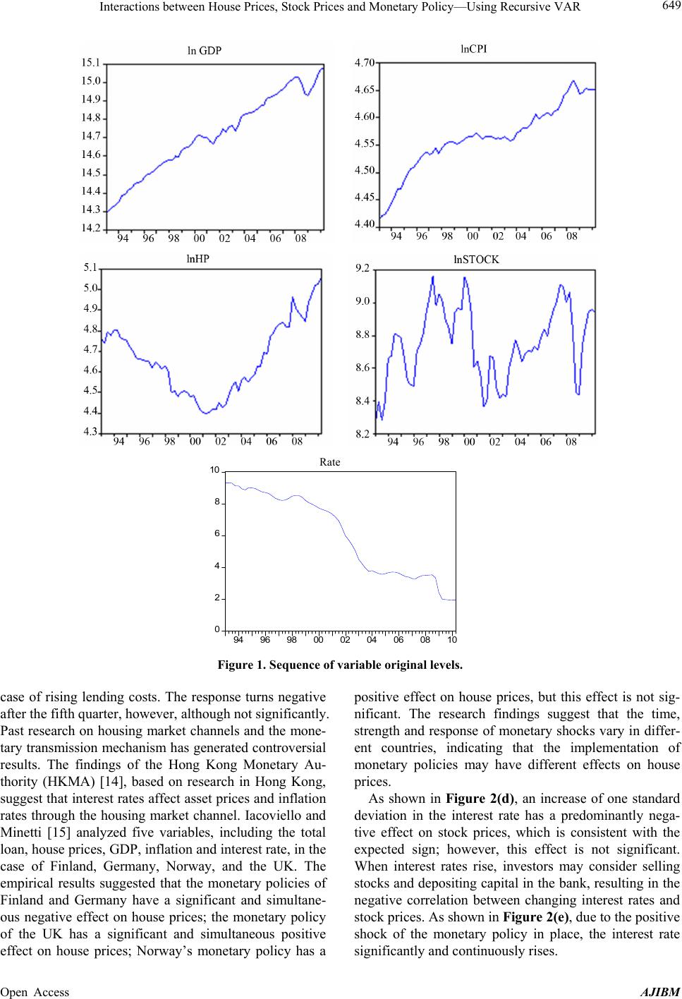

Interactions between House Prices, Stock Prices and Monetary Policy—Using Recursive VAR

Open Access AJIBM

649

94 96 98 00 02 04 06 08 10

Rate

Figure 1. Sequence of variable original levels.

case of rising lending costs. The response turns negative

after the fifth quarter, however, although not significantly.

Past research on housing market channels and the mone-

tary transmission mechanism has generated controversial

results. The findings of the Hong Kong Monetary Au-

thority (HKMA) [14], based on research in Hong Kong,

suggest that interest rates affect asset prices and inflation

rates through the housing market channel. Iacoviello and

Minetti [15] analyzed five variables, including the total

loan, house prices, GDP, inflation and interest rate, in the

case of Finland, Germany, Norway, and the UK. The

empirical results suggested that the monetary policies of

Finland and Germany have a significant and simultane-

ous negative effect on house prices; the monetary policy

of the UK has a significant and simultaneous positive

effect on house prices; Norway’s monetary policy has a

positive effect on house prices, but this effect is not sig-

nificant. The research findings suggest that the time,

strength and response of monetary shocks vary in differ-

ent countries, indicating that the implementation of

monetary policies may have different effects on house

prices.

As shown in Figure 2(d), an increase of one standard

deviation in the interest rate has a predominantly nega-

tive effect on stock prices, which is consistent with the

expected sign; however, this effect is not significant.

When interest rates rise, investors may consider selling

stocks and depositing capital in the bank, resulting in the

negative correlation between changing interest rates and

stock prices. As shown in Figure 2(e), due to the positive

shock of the monetary policy in place, the interest rate

significantly and continuously rises.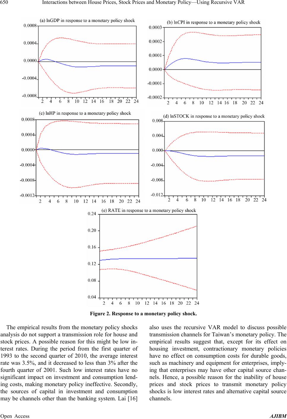

Interactions between House Prices, Stock Prices and Monetary Policy—Using Recursive VAR

650

Figure 2. Response to a monetary policy shock.

The empirical results from the monetary policy shocks

analysis do not support a transmission role for house and

stock prices. A possible reason for this might be low in-

terest rates. During the period from the first quarter of

1993 to the second quarter of 2010, the average interest

rate was 3.5%, and it decreased to less than 3% after the

fourth quarter of 2001. Such low interest rates have no

significant impact on investment and consumption lend-

ing costs, making monetary policy ineffective. Secondly,

the sources of capital in investment and consumption

may be channels other than the banking system. Lai [16]

also uses the recursive VAR model to discuss possible

transmission channels for Taiwan’s monetary policy. The

empirical results suggest that, except for its effect on

housing investment, contractionary monetary policies

have no effect on consumption costs for durable goods,

such as machinery and equipment for enterprises, imply-

ing that enterprises may have other capital source chan-

nels. Hence, a possible reason for the inability of house

prices and stock prices to transmit monetary policy

shocks is low interest rates and alternative capital source

hannels. c

Open Access AJIBM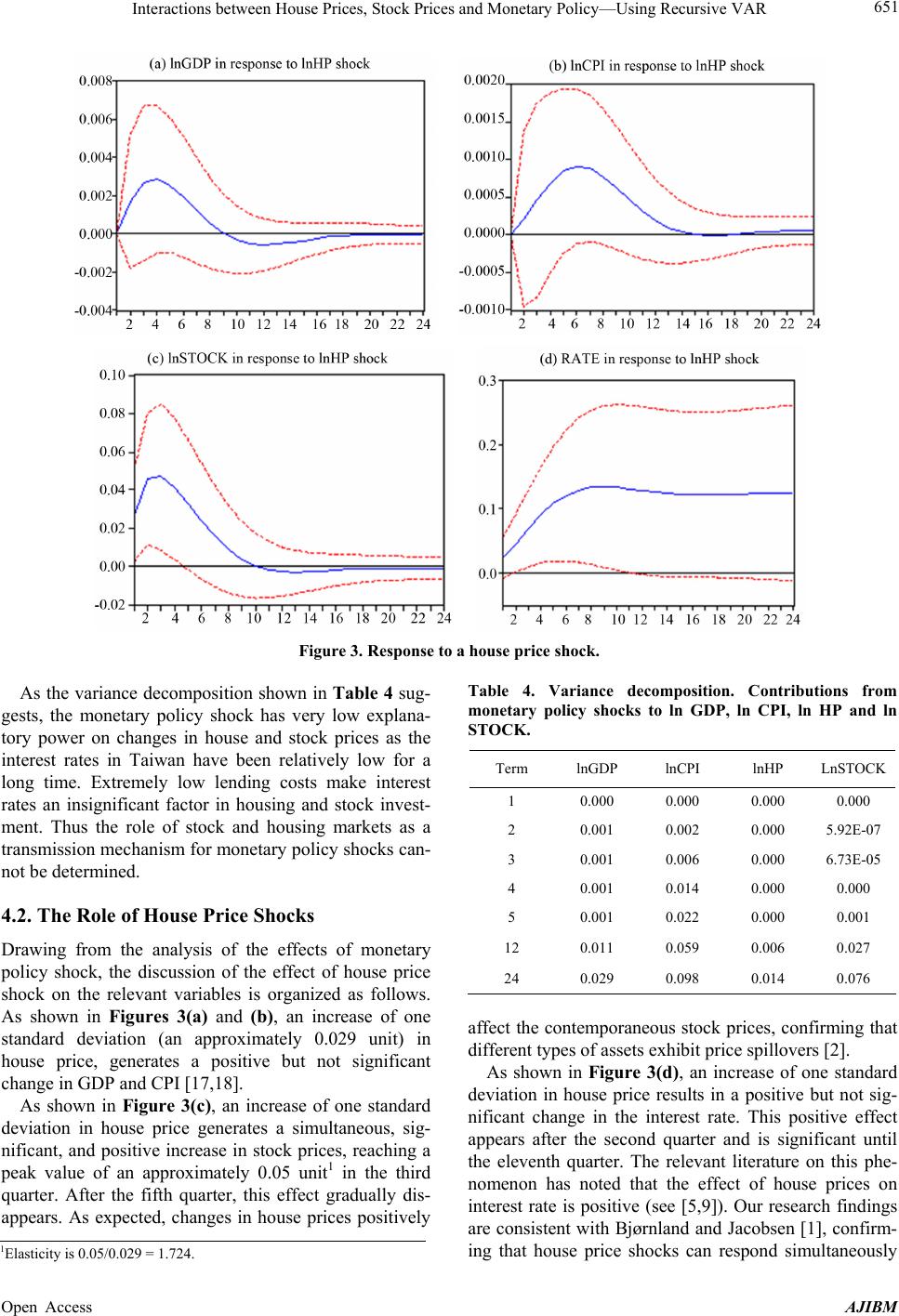

Interactions between House Prices, Stock Prices and Monetary Policy—Using Recursive VAR 651

Figure 3. Response to a house price shock.

As the variance decomposition shown in Table 4 sug-

gests, the monetary policy shock has very low explana-

tory power on changes in house and stock prices as the

interest rates in Taiwan have been relatively low for a

long time. Extremely low lending costs make interest

rates an insignificant factor in housing and stock invest-

ment. Thus the role of stock and housing markets as a

transmission mechanism for monetary policy shocks can-

not be determined.

4.2. The Role of House Price Shocks

Drawing from the analysis of the effects of monetary

policy shock, the discussion of the effect of house price

shock on the relevant variables is organized as follows.

As shown in Figures 3(a) and (b), an increase of one

standard deviation (an approximately 0.029 unit) in

house price, generates a positive but not significant

change in GDP and CPI [17,18].

As shown in Figure 3(c), an increase of one standard

deviation in house price generates a simultaneous, sig-

nificant, and positive increase in stock prices, reaching a

peak value of an approximately 0.05 unit1 in the third

quarter. After the fifth quarter, this effect gradually dis-

appears. As expected, changes in house prices positively

Table 4. Variance decomposition. Contributions from

monetary policy shocks to ln GDP, ln CPI, ln HP and ln

STOCK.

Term lnGDP lnCPI lnHP LnSTOCK

1 0.000 0.000 0.000 0.000

2 0.001 0.002 0.000 5.92E-07

3 0.001 0.006 0.000 6.73E-05

4 0.001 0.014 0.000 0.000

5 0.001 0.022 0.000 0.001

12 0.011 0.059 0.006 0.027

24 0.029 0.098 0.014 0.076

affect the contemporaneous stock prices, confirming that

different types of assets exhibit price spillovers [2].

As shown in Figure 3(d), an increase of one standard

deviation in house price results in a positive but not sig-

nificant change in the interest rate. This positive effect

appears after the second quarter and is significant until

the eleventh quarter. The relevant literature on this phe-

nomenon has noted that the effect of house prices on

interest rate is positive (see [5,9]). Our research findings

are consistent with Bjørnland and Jacobsen [1], confirm-

ng that house price shocks can respond simultaneously i

1Elasticity is 0.05/0.029 = 1.724.

Open Access AJIBM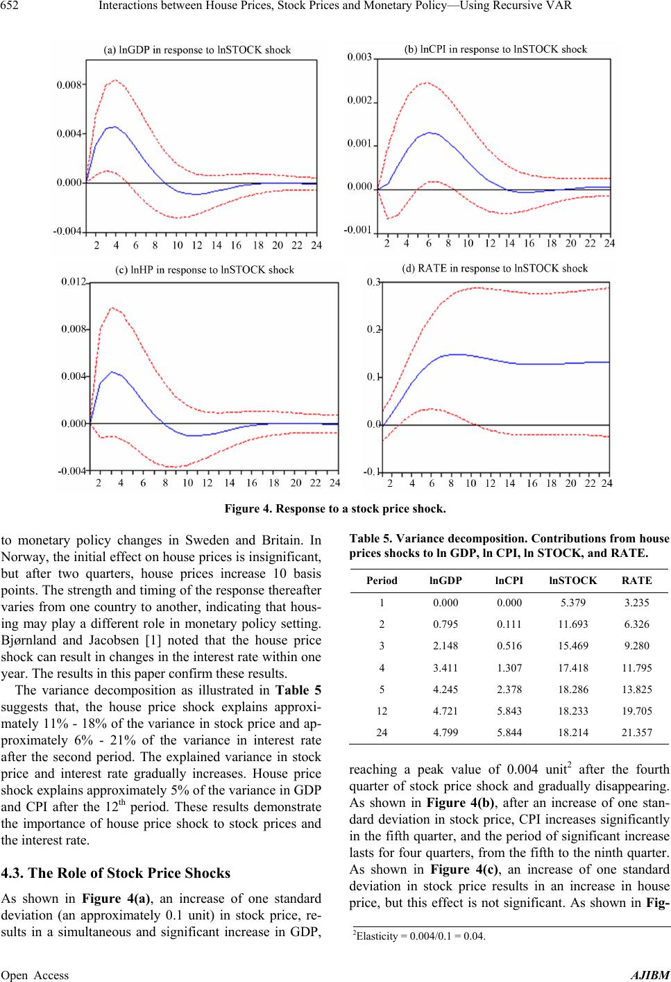

Interactions between House Prices, Stock Prices and Monetary Policy—Using Recursive VAR

652

Figure 4. Response to a stock price shock.

to monetary policy changes in Sweden and Britain. In

Norway, the initial effect on house prices is insignificant,

but after two quarters, house prices increase 10 basis

points. The strength and timing of the response thereafter

varies from one country to another, indicating that hous-

ing may play a different role in monetary policy setting.

Bjørnland and Jacobsen [1] noted that the house price

shock can result in changes in the interest rate within one

year. The results in this paper confirm these results.

The variance decomposition as illustrated in Table 5

suggests that, the house price shock explains approxi-

mately 11% - 18% of the variance in stock price and ap-

proximately 6% - 21% of the variance in interest rate

after the second period. The explained variance in stock

price and interest rate gradually increases. House price

shock explains approximately 5% of the variance in GDP

and CPI after the 12th period. These results demonstrate

the importance of house price shock to stock prices and

the interest rate.

4.3. The Role of Stock Price Shocks

As shown in Figure 4(a), an increase of one standard

deviation (an approximately 0.1 unit) in stock price, re-

sults in a simultaneous and significant increase in GDP,

Table 5. Variance decomposition. Contri butions from house

prices shocks to ln GDP, ln CPI, ln STOCK, and RATE.

Period lnGDP lnCPI lnSTOCK RATE

1 0.000 0.000 5.379 3.235

2 0.795 0.111 11.693 6.326

3 2.148 0.516 15.469 9.280

4 3.411 1.307 17.418 11.795

5 4.245 2.378 18.286 13.825

12 4.721 5.843 18.233 19.705

24 4.799 5.844 18.214 21.357

reaching a peak value of 0.004 unit2 after the fourth

quarter of stock price shock and gradually disappearing.

As shown in Figure 4(b), after an increase of one stan-

dard deviation in stock price, CPI increases significantly

in the fifth quarter, and the period of significant increase

lasts for four quarters, from the fifth to the ninth quarter.

As shown in Figure 4(c), an increase of one standard

deviation in stock price results in an increase in house

price, but this effect is not significant. As shown in Fig-

2Elasticity = 0.004/0.1 = 0.04.

Open Access AJIBM

Interactions between House Prices, Stock Prices and Monetary Policy—Using Recursive VAR 653

ure 4(d), an increase of one standard deviation in stock

price results in a simultaneous, significant increase in the

interest rate from the third to the tenth quarter, reaching a

peak value of approximately 0.15 units in the ninth quar-

ter after the shock. From the perspective of point estima-

tion, the effect seems to be permanent, but it becomes

insignificant after the tenth quarter.

The variance decomposition illustrated in Table 6

suggests that the variance in GDP, CPI, house price and

interest rate attributable to the stock price shock is low

at first but gradually increases with time. The ranking

by explanatory variance is interest rate, GDP, CPI and

house price, indicating that stock price shocks have a

significant long-term impact on interest rate, GDP and

CPI.

5. Conclusions and Suggestions

This study uses a recursive VAR model to analyze the

effect of monetary policy shocks and the role of house

price and stock price shocks. The empirical results

suggest that contractionary monetary policy shock has no

significant impact on GDP, CPI, house prices and stock

prices. The role of house prices and stock prices as a

transmission mechanism for monetary policy shock

cannot be confirmed.

The findings on the effect of house price changes

suggest that stock prices will be simultaneously and

positively affected when house prices increase but that

this effect gradually disappears after the fifth quarter.

Increases in house prices result in simultaneous increases

in the interest rate, and this effect becomes significant

after the second quarter and lasts until the eleventh

quarter. These results are consistent with Bjørnland and

Jacobsen [1]. The results from the stock price shock

analysis suggest that GDP significantly increases with

increases in stock price, but this effect lasts only until

the fifth quarter. Increases in stock prices positively and

significantly affect CPI. An effect lasts for four quarters

from the fifth to the ninth quarter. House prices are

Table 6. Variance decomposition. Contributions from stock

price shocks to lnGDP, lnCPI, lnHP, and RATE.

Term lnGDP lnCPI lnHP RATE

1 0.000 0.000 0.000 0.078

2 2.651 0.056 1.074 1.364

3 6.491 0.656 2.590 4.694

4 9.676 2.193 3.742 8.673

5 11.564 4.451 4.327 12.358

12 12.314 11.454 4.678 22.449

24 12.438 11.436 4.738 23.961

positively affected by increases in stock prices, but this

effect is not significant. As stock prices increase, the

interest rate simultaneously increases, and this effect is

significant from the third to the tenth quarter, becoming

insignificant after the tenth quarter.

This analysis in this paper assumed a traditional closed

economic system. However, because Taiwan is a small

open economy, the interaction between exchange rate

and monetary policy might be significant, as previous

studies suggest [19-21].

Exchange rates and international crude oil prices may

be added as the foreign economic variables. Given that

mainland China, the US and Taiwan are closely related

in terms of economy, future studies may wish to include

data on China and the US in the analysis. Additionally,

this paper uses the weighted average lending rate as a

proxy variable for monetary policy. However, the

weighted average lending rate published by the Central

Bank is not entirely subject to the control of monetary

policy designed to regulate supply and demand in capital

markets. Hence, future studies may wish to use monetary

supply or non-borrowed money supply as a proxy vari-

able for monetary policy.

REFERENCES

[1] H. C. Bjørnland and D. H. Jacobsen, “The Role of House

Prices in the Monetary Policy Transmission Mechanism

in Small Open Economies,” Journal of Financial Stability,

Vol. 6, No. 4, 2010, pp. 218-229.

http://dx.doi.org/10.1016/j.jfs.2010.02.001

[2] International Monetary Fund, “Lessons for Asset Price

Fluctuations Form Monetary Policy,” World Economic

Outlook, 2009, pp. 93-120.

[3] R. Rigobon and B. Sack, “The Impact of Monetary Policy

on Asset Prices,” Journal of Monetary Economics, Vol.

51, No. 8, 2004, pp. 1553-1575.

http://dx.doi.org/10.1016/j.jmoneco.2004.02.004

[4] J. Zettelmeyer, “The Impact of Monetary Policy on the

Exchange Rate: Evidence from Three Small Open

Economies,” Journal of Monetary Economics, Vol. 51,

No. 3, 2004, pp. 635-652.

http://dx.doi.org/10.1016/j.jmoneco.2003.06.004

[5] B. S. Bernanke and K. N. Kuttner, “What Explains the

Stock Market’s Reaction to Federal Reserve Policy?” The

Journal of Finance, Vol. 60, No. 3, 2005, pp. 1221-1257.

[6] K. E. Case, J. M. Quigley and R. J. Shiller, “Comparing

Wealth Effects: The Stock Market Versus the Housing

Market,” Advances in Macroeconomics, Vol. 5, No. 1,

2005, pp. 1-34. http://dx.doi.org/10.2202/1534-6013.1235

[7] B. S. Bernanke and A. S. Blinder, “The Federal Funds

Rate and the Channels of Monetary Transmission,” Ameri-

can Economic Review, Vol. 82, No. 4, 1992, pp. 901-921.

[8] N. Girouard and S. Blöndal, “House Prices and Economic

Activity,” OECD Economics Department Working Pa-

pers, No. 279, 2001.

Open Access AJIBM

Interactions between House Prices, Stock Prices and Monetary Policy—Using Recursive VAR

Open Access AJIBM

654

[9] C. Goodhart and B. Hofmann, “Asset Prices, Financial

Conditions, and the Transmission of Monetary Policy,”

Paper Presented at Conference on Asset Prices, Exchange

Rates, and Monetary Policy, 2001.

[10] J. J. Rotemberg and M. Woodford, “An Optimization-

Based Econometric Framework for the Evaluation of

Monetary Policy,” NBER Macroeconomics Annual, Vol.

12, 1997, pp. 297-346. http://dx.doi.org/10.2307/3585236

[11] E. O. Svensson Lars, “Inflation Forecast Targeting:

Implementing and Monitoring Inflation Targets,” Euro-

pean Economic Review, Vol. 41, No. 6, 1997, pp. 1111-

1146. http://dx.doi.org/10.1016/S0014-2921(96)00055-4

[12] A. Elbourne and J. de Haan, “Financial Structure and

Monetary Policy Transmission in Transition Countries,”

Journal of Comparative Economics, Vol. 34, No. 1, 2006,

pp. 1-23. http://dx.doi.org/10.1016/j.jce.2005.11.004

[13] E. O. S. Lars, “Inflation Forecast Targeting: Implement-

ing and Monitoring Inflation Targets,” European Econo-

mic Review, Vol. 41, No. 6, 1997, pp. 1111-1146.

http://dx.doi.org/10.1016/S0014-2921(96)00055-4

[14] Hong Kong Monetary Authority, “The Housing Market

Channel of the Monetary Transmission Mechanism in

Hong Kong,” Bank for International Settlements, Vol. 35,

2008, pp. 221-233.

[15] M. Iacoviello and R. Minetti, “The Credit Channel of

Monetary Policy: Evidence from the Housing Market,”

Journal of Macroeconomics, Vol. 30, No. 1, 2008, pp.

69-96. http://dx.doi.org/10.1016/j.jmacro.2006.12.001

[16] H. Z. Lai, “Discussion on Credit Transmission Mecha-

nism Channels of Taiwan’s Monetary Policy,” Taiwan

Economics Inquiry, Vol. 38, No. 1, 2002, pp. 57-95.

[17] R. S. Chirinko, L. de Haan and E. Sterken, “Asset Price

Shocks, Real Expenditures, and Financial Structure: A

Multi-Country Analysis,” University of Groningen, CCSO

Centre for Economic Research, Groningen, 2004.

[18] A. Elbourne, “The UK Housing Market and the Monetary

Policy Transmission Mmechanism: An SVAR Approach,”

Journal of Housing Economics, Vol. 17, No. 1, 2007, pp.

65-87. http://dx.doi.org/10.1016/j.jhe.2007.09.002

[19] J. Faust and J. H. Rogers, “Monetary Policy’s Role in

Exchange Rate Behavior,” Journal of Monetary Econo-

mics, Vol. 50, No. 7, 2003, pp. 1403-1424.

http://dx.doi.org/10.1016/j.jmoneco.2003.08.003

[20] H. C. Bjørnland, “Monetary Policy and Exchange Rate

Overshooting: Dornbusch Was Right After All,” Journal

of International Economics, Vol. 79, No. 1, 2009, pp. 64-

77. http://dx.doi.org/10.1016/j.jinteco.2009.06.003

[21] H. C. Bjørnland and J. I. Halvorsen, “How Does Mone-

tary Policy Respond to Exchange Rate Movements?”

Norges Bank Working Paper, 2008.

http://dx.doi.org/10.1111/obes.12014