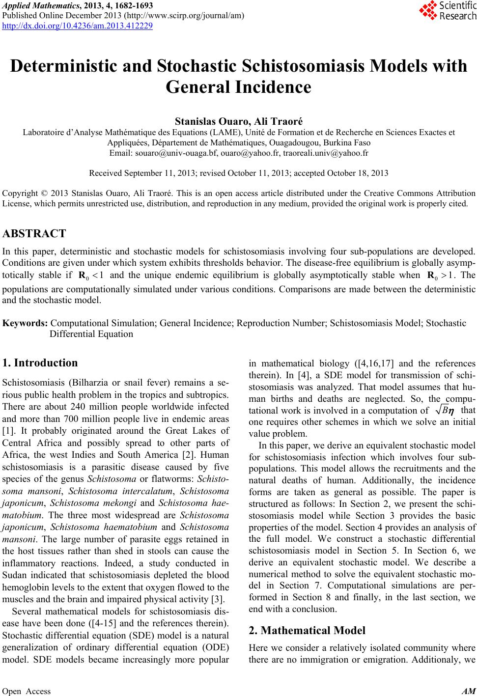Applied Mathematics, 2013, 4, 1682-1693
Published Online December 2013 (http://www.scirp.org/journal/am)
http://dx.doi.org/10.4236/am.2013.412229
Open Access AM
Deterministic and Stochastic Schistosomiasis Models with
General Incidence
Stanislas Ouaro, Ali Traoré
Laboratoire d’Analyse Mathématique des Equations (LAME), Unité de Formation et de Recherche en Sciences Exactes et
Appliquées, Département de Mathématiques, Ouagadougou, Burkina Faso
Received September 11, 2013; revised October 11, 2013; accepted October 18, 2013
Copyright © 2013 Stanislas Ouaro, Ali Traoré. This is an open access article distributed under the Creative Commons Attribution
License, which permits unrestricted use, distribution, and reproduction in any medium, provided the original work is properly cited.
ABSTRACT
In this paper, deterministic and stochastic models for schistosomiasis involving four sub-populations are developed.
Conditions are g iven under which system exhibits thresho lds behavior. The disease-free equ ilibrium is globally asymp-
totically stable if and the unique endemic equilibrium is globally asymptotically stable when . The
populations are computationally simulated under various conditions. Comparisons are made between the deterministic
and the stochastic model.
01R01R
Keywords: Computational Simulation; General Incidence; Reproduction Number; Schistosomiasis Model; Stochastic
Differential Equation
1. Introduction
Schistosomiasis (Bilharzia or snail fever) remains a se-
rious public health problem in th e tropics and subtropics.
There are about 240 million people worldwide infected
and more than 700 million people live in endemic areas
[1]. It probably originated around the Great Lakes of
Central Africa and possibly spread to other parts of
Africa, the west Indies and South America [2]. Human
schistosomiasis is a parasitic disease caused by five
species of the genus Schistosoma or flatworms: Schisto-
soma mansoni, Schistosoma intercalatum, Schistosoma
japonicum, Schistosoma mekongi and Schistosoma hae-
matobium. The three most widespread are Schistosoma
japonicum, Schistosoma haematobium and Schistosoma
mansoni. The large number of parasite eggs retained in
the host tissues rather than shed in stools can cause the
inflammatory reactions. Indeed, a study conducted in
Sudan indicated that schistosomiasis depleted the blood
hemoglobin levels to the extent that oxygen flowed to the
muscles and the brain and impaired physical activity [3].
Several mathematical models for schistosomiasis dis-
ease have been done ([4-15] and the references therein).
Stochastic differential equation (SDE) model is a natural
generalization of ordinary differential equation (ODE)
model. SDE models became increasingly more popular
in mathematical biology ([4,16,17] and the references
therein). In [4], a SDE model for transmission of schi-
stosomiasis was analyzed. That model assumes that hu-
man births and deaths are neglected. So, the compu-
tational work is invo lved in a computation of B

that
one requires other schemes in which we solve an initial
value problem.
In this paper, we derive an equivalent stochastic model
for schistosomiasis infection which involves four sub-
populations. This model allows the recruitments and the
natural deaths of human. Additionally, the incidence
forms are taken as general as possible. The paper is
structured as follows: In Section 2, we present the schi-
stosomiasis model while Section 3 provides the basic
properties of the model. Section 4 provides an analysis of
the full model. We construct a stochastic differential
schistosomiasis model in Section 5. In Section 6, we
derive an equivalent stochastic model. We describe a
numerical method to solve the equivalent stochastic mo-
del in Section 7. Computational simulations are per-
formed in Section 8 and finally, in the last section, we
end with a conclusion.
2. Mathematical Model
Here we consider a relatively isolated community where
there are no immigration or emigration. Additionaly, we

S. OUARO, A. TRAORÉ 1683
suppose that all newborns are susceptible and the infec-
tion does not imply death or isolation of the different
hosts.
Then, according to Figure 1, we obtain the following
system of four differential equations




d,,
d
d,,
d
d,,
d
d,,
d
shhs is i
iis hii
ssss is
iis si
HbdH fSHH
t
HfSH dHH
t
SbdSgHS
t
SgHSdS
t


 






 





(1)
where

s
H
t is the size of the susceptible human
population;

i
H
t

St is the size of the infected human population;
s

St is the size of the susceptible snails;
i
b is the size of the infected snails;
h is the recruitment rate of human hosts;
s
b is the recruitment rate of snails;
h
osts
d is the per capita natural death rate of human
h;
s
d is the per capita natural death rate of snails;

is the treatment rate of human hosts;
f
is the infection function of susceptible human due
to infected snails;
g
is the infection function of susceptible snails due to
in nctions fected human.
We assume that the fu
f
and
g
satisfies the
fopllowing assumtions.
H1
f
and
g
are nonnegative functions on the
nort.
H For all ,
1
C
nnegative o,
i
S
than
2
f

4
,,
sis
HHS 
,0 

0, 0
si
H fS and
 
0,,0 0
si
gS gH.
Remark 2.1
f
and
g
are two incidence functions
ich explain the contact between two species. Therefore,
is no infected in the human and snail populations, then
the incidence functions are equal to zero. The incidence
functions are also equal to zero when there is no sus-
ceptible in the human and snail populations.
3. Model Basic Properties
are nnegve. Note also that when there

no ati
In this section, we study the basic properties of the solu-
tions of system (1).
Theorem 3.1 [18] Let : be a dif-
ferentiable function and let L

n

X
x be a vector field. Let
a

 and let



xa:
n
Gx L

 be such that


Lx 0

 for all






1: n
x
LaxLxa


 . If



0Xx Lx
for all


1
x
L
aG then, the set is positively in-
variant.
Lemma 3.2 The system Equation (1) preserve the
positivity of solutions.
proof. We start by proving that




4
,,,; 0
sisi i
HHSS H

 is positively invariant.
For that, let


,,,
s
isi
x
HHSS and

i
Lx H

.


Lx is differentiable and
for all

0Lx
 
0, 1,0,0




4
:0x
1
0xLxL


.
The vector field on the set




4
,,,; 0
sisi i
HHSS H

 is




,
,.
hishs
is
sss
si
bfSH dH
fSH
Xx bdS
dS


















(2)
We obtain



 
,
is
Xx LxfSH0

 . Then,
using Theorem 3.1, we conclude that




4
,,,; 0
sisi i
HHSS H

 is positively invariant.
Similarly we prove that




4
,,,; 0
sisi s
HHSS H,




4
,,,; 0
sisi s
HHSS S

 and




4
,,,; 0
sisi i
HHSS S

 are positively invariant 
Lemma 3.3 Each nonnegative solution of model
system (1) is bounded.
wh
f
and
g
Figure 1. Transfer diagram.
Open Access AM

S. OUARO, A. TRAORÉ
1684
Proof. Let
 
si
H
tHtHt

si
S t. Then, adding t
second two Equations
and
he first two equa-
pectively,
we get
 
StSt
tions and the of (1) res
and .
hh ss
H
bdH SbdS

 (3)
According to [19], it follows that
 
 
0e
and0e ,
h
s
dt
hh
dt
ss
ss
bb
St S
dd



 


(4)
where 0 and
hh
bb
HtH
dd

 


 
00
si
HH H
 
000
si
SS S.
,

Thus
 
lim
t and lim
hs
t
hs
bb
Ht St
dd
 
 (5)
Corollary 3.4 The set
    
 
4
,,
sis
KHtHtS



, ;
0,0
i
hs
si si
hs
tSt
bb
Ht HtStSt
dd







is invariant and attracting for system (1).
Theorem 3.5 For every nonzero, nonnegative initial
ist for all time
dard uments since the right-hand side of system (1) is
lo
nd
analyze the eventual equilibria. For that, let us denote
value, solutions of model system (1) ex
0.
Proof. Local existence of solutions follows from stan-
arg
t
cally Lipschitz. Global existence follows from the a
priori bounds. 
4. Reproduction Number and Equilibria
Analysis
In this section, we define the reproduction number a
 
 
12
,, ,.
is is
is
gg
12
,, ,,
is is
is
ff
fSHf SH
SH
g
HS gHS
HS



System (1) has a disease-free equilibrium (DFE) given
by




00
,0,,0,0,,0 .
hs
bb
EHS 
DFE s shs
dd


Proposition 4.1 The reproduction number fr system
(1) is o


00
0, 0,
11
0.
ss
sh
f
HgS
dd

 R
Proof. We use the method in [20] to compute the
reproduction number
Let 0
R.


12
,
X
XX, where

1,
s
s
X
HS

=,
ii
is the
healthand y population 2
X
HS , the infected
population.


1
,hi i
is idH H
fSH
H
XS

 
 
 



12
,
.
si is
idS
gHS
X


 

12
,,XX X 
Then,








1
11
2
1
2
00,
,0 0, 0
0
and ,0.
0
s
s
h
s
fH
FX
gS
X
d
VX d
X











 





Hence,



1
11
1
0,
100
and .
10,
00
s
hs
s
sh
fH
dd
VFV
gS
dd




 





 
 

 
The basic reproduction number is defined as the
dominant eigenvalue of matrix 1
F
V [20].
Therefore,


00
11
0
0, 0,
ss
sh
dd


The basic reproduction numvaluate
fHgS
R
ber ethe average
nunfections generated by a single infected
individual in a completely susceptible population.
Using Theorem 2 in [20], the following result is estab-
lished.
mber of new i
Lemma 4.2 If 01

R, then
D
FE
E is locally
asymptotically stable.
Proof. Using the assumption H2, it follows that


0, 0fH
2s

and


0, 0gS for all
2s
s
H
and s S.
Then, the linearization of system (1) at
D
FE
E gives the
following equation









11
0
sh
dd
f00 ,0, 0.
ss
H
gS
hs
dd




  




(6)
We can see that all solution

of Equation (6) have
negative real part. Indeed, the Equation (6) has negative
roots h
d


,
s
d


 and oots are given by ther ro





0
11
0, 0,
shs s
dd fHgS  

0
. (7)
Now, we suppose that there exts at least one root 1 is

of the Equation (7) which have positive real part.
According to Proposition 4.1, it follows that
Open Access AM

S. OUARO, A. TRAORÉ 1685

0
11
0 0
s
fHg


02
0
, ,.
ssh
S dd

R
Since , we obtain
0<1R


00
11 11
0, 0,
sssh sh
HgS dddd.f




This show that the Equation (7) cannot have roots with
positive real part. Hence,
D
FE
Eing to T is locally
asymptotically stable accordheorem 2 in [20] 
et us abal behavior of the DFE.
The global stability of the DFE will be studied using the
basic reproduction number . We first make the
fo
Now, lnalyze the glo
0
R
llowing additional assumption.
H3 For all

4
,,,
sis
HHSS  ,


0
1
,0,
is si
i
f
SHfH S and


0
1
,0,
iss i
g
HSgS H.
Theorem 4.3 The disease-free equilibrium is globally
asymptotically stable in
K
whenever 0<1R.
Proof. The proof is basedon using a comparison
theorem [21]. Note that the equations of the infected
co system (1) can be essed as mponents inxpre

,
d
i
i
i
FV S
S
 
 

(8)
d
di
HH
t

 
dt 
where
F
and V, are defined in the proof of Pro-
position 1.
Using the fact that all the eigenvalues of the matrix
F
V
whenev
eigenvalues
have negative real parts, it follows that the
linearized differential inequality syste
er . Indeed, we can see that all
m (8) is stable
0<1R

of the matrix
F
V satisfy Equation
th(7). Bye sameasoning as in the proof of Lemma 4.2
we deduce that, the eigenvalues of the matrix
re
F
V

have negative real parts since 0<1R.
T,
 

hus

,0,0
ii
HtSt  as t for the
system (8). Consequently, by a standard comparison
theorem [21
   
,0,0
ii
tSt  as t and
substituting 0
ii
HS into system (1) gives
0
], H
s
s
H
H and 0
s
s
SS as t.
Thus,
 

 

00
,,, ,0,,
sisi s
HtHtStStH
as t for 0<1R. The0
s
S
refore,
D
FE
E is globally
lly stable if 0<1R. 
as icymptot
Lemma 4.4 If 01R then,
a
D
FE
E is unstable and
there exists a unim qendemic equilibriue u

,,,
s
i
EHHS
Proof Let si
S
.
.

,,,
s
is
ES . It follows that
i
SHHE is
a positive equilibrium if and only if




,0,
hhs is
bfSH H
H

 
,0
,
0,
ihi
s
fSH H 


 (9)
,
,0 .
i
s i
ss is
is si
dH
d
bdSgHS
HS dS





wo equations of sys-
tem (9) respectively, we get
g



Adding the first two and the last t
0 and0.
hhshissssi
bdHdHb dSdS

 
Then,
and .
hhi ssi
ss
hs
bdH bdS
HS
dd


Let


,,
,, .
hhi
iii h
ssi
hiisi
s
bdH
hS HfSd
bdS
dHgH dS
d









 




on is continuous and so
sy (9) hold whenever

We can see that the functi
stem h

,0hS . Therefore any
zero of h in the set
ii
H
0, 0,
sh
sh
bb
dd







where i
H
and
i
S are positives corresponds to an endemic e.
According to H2,
quilibrium


0,00h

and ,0
sh
bb
h
sh
dd


olution of equ

Then, in order to have a sation 0h
.

in
0, 0,
sh
sh
dd

 
 
, h 0. This lea to
bb


must increase at ds

2
d0,0 0, h (10)
dX
where 2
X
is defined in the proof of Proposition 4.1.
We can see that
 
00
0, , 0,.
sh ss

11
2
d
d
h
f
Hd gSd   
X
It follows from inequality (10) that




0
1
1
0
1
0
1
0, 0
or 0,0
and 0,0.
sh
ss
sh
ss
fHd
gSd
fHd
gSd







0
0, 0and

 

0
0,fHg
Which implies that
0
11
0, 1
ss
sh
S
dd


, that is

To study the global behaviour of this endemic
equilibrium, we second make this additional assumption.
H4 For all
01R.


4
,,,
sisi
HHSS  ,
Open Access AM

S. OUARO, A. TRAORÉ
Open Access AM
1686




,
1,
,
and 1.
,
is
si
i
is
s
is
s
i
i
is
s
fSH
HS
S
fSH
H
gHS
SH
H
gHS
S









 
and



 






,,
,,
,,
,.
s
hsi sss
i
hii sii
s
ssis ss
i
siis ii
H
t
VtgHSHh H
Ht
VtgHSHhH
St
VtfSHSh S
St
Vtf S HShS















(11) 
*
(14)
Theorem 4.5 When 0

 and 01R, the endemic
equilibrium E is globally asymptotically stable in K.
when 1R, We can see that *
:h


 has the strict global
minimun


10h

. Thus,
hs with equality if and only
if 0,VV0,
hi ss
V0, 0
si
V
,,
s
siiss
H
HH HSS

 and ii . We will
study the behaviour of the Lyapunov function
Proof. If wem
ere exists a e consider the syst (1) thunique endemic equilibrium 0
E. We now
ic establish the global asymptotic stability of this endem
equilibrium. Evaluating both sides of (1) at E with
0


SS
gives


.
hs hi ss si
Vt VVVV (15)





,,
,,
,,
,.
hhs is
hiis
sss is
sii s
bdHfSH
dHfS H
bdSgHS
dSg HS









We can see that


0Vt with equality if and only if



 
1,1,1 and1.
sisi
sisi
Ht Ht StSt
HHS S


(12)
(1

The derivatives of and ,,
hs hi ss
VVV
s
i will be
calculated separately and then combined to get the
V
Let

1lnhx xx 3) desired quantity d
d
V
t.
 
 
,1,.
s
ishhsi s
s
H
Sb dHfSH
tH




UsiEquation of (12) to replace gives
dd
,1
dd
hsss
is s
VHH
gHS gH
tH




ng the first h b
  







2

 
 


2
d,1, ,
d
,
,,,11
,
,,
,,,1 .
,,
hs s
ishssi sis
s
ss is s
hisis is
s s
is
ss is is
ss
hisisss
is is
VH
gHSd HHfSHfSH
tH
HH fSH H
dgHSgH Sf S H
HH
fSH
HH fSH fSH
HH
dgHSgH Sf S H
HHH
fSH fSH

 





 






 


By adding and substracting the quantity
is
s



,
1ln ,
is
s
s
is
fSH
H
H
fSH
, we obtain















2
2
d,1ln
,,, ,
1ln 1ln
,,, ,
,
,,,
ss ss
is ss
isis isis
ss
ss
isis isis
ss i
s
hisis is
ss
HH
VHH
gS HHH
fSHfSH fSHfSH
HH
HH
fSHfSH fSHfSH
HH fSH
H
dgHSgH Sf S Hhh
HH

 




 

 
 
 

 


 



,,
dhs hi
s is
s
dgH SH Sf
tH
 



,.
,,
sis
s
s
is is
fSH H
hH
fSH fSH


 

  

 


 

(16)


S. OUARO, A. TRAORÉ 1687
d
dhi
V
t. Next, we calculate



 


dd
,1(,)1,
d
,
,1 ,.
,
hiiii
isisishi
ii
is
ii
isi shi
ii
is
VHHH
g
HSgHSfSHdH
tHdtH
fSH
HH
gHS fSHdH
HH
fSH

 





 




hi
dH Using the second Equation of (12) to replace gives


 




,,
d,,1,,1
d,,
isis is
hiiii i
is isis is
ii ii
isis is
fSHfSH fSH
VHH HH
fSHgHSfSHgHS
tHHHH
fSHfSH fSH
 

 


 

 
,
.
,




By adding and substracting the quantity



,
1ln ,
is i
i
is
fSH
H
H
fSH
, we obtain








 




,,
d,, 1ln1ln
d,,
, ,
n, ,, ,
is is
hii iii
is isii ii
is is
isis is
ii
is isii
is isisis
fSHfSH
VHHHH
fSHgHS
tHHHH
fSHfSH
SHfSHfSH
HH
fSHgHShhh
HH
SHfSHfSH









 

  
 

 

 

.



,,
1l
,,
is
fSH f
fSH f




 






(17)
Now, we calculate d
d
s
s
V
t.

 
dd
,1 ,1,
dd
sss ss
isissssis
ss
VSSS
fSHfSHb dSgHS
tStS
 

 
 
.
Using the third Equation of (12) to replace
s
bes giv
 














2
2
d,1, ,
d
,
,,,11
,,
,,,1 .
,,
ss s
isss sisis
s
ss is s
is is
ss is is
ss
sisis is
sss
is is
VS
fSHdSSgHSgHS
tS
SS gHS S
df SHf SHgH SS
S
SS gHSgHS
SS
df SHf SHgH S
SSS
gHSgHS







 









By adding and substracting the quantity
,
si s s
sis
S
gH





,
1ln ,
is
s
s
is
gHS S
S
gHS
, we obtain














2
d,1ln
,,,,
1ln 1ln
,,,,
,
,,,
ss ss
sisis is
sss
isis isis
ss
ss
isis isis
i
s
sisisis
ss
SS
VSS
Hf S HgH S
S SS
gHSgHSgHSgHS
SS
SS
gHSgHSgHSgHS
gHS
S
df SHfSHgH Shh
SS









 









,,
dss df S t

2
ss
SS



,.
,,
sis
s
s
is is
gHS S
hS
gHS gHS


 

  

 


 

(18)

Open Access AM

S. OUARO, A. TRAORÉ
Open Access AM
1688
After that, we evaluate d
d
s
i
V
t.




 


dd
,1
dd
,1 ,
,
,1 ,.
sii i
is i
i
isis si
i
is
ii
isis si
,
i
VSS
fSH
tSt
S
fSHgHS dS
S
gHS
SS
fSH gHSdS
i
S

is
S





 





 
 gHS

Using the last Equation of (12) to replace










,
d,,1
d,
,,
,,
1.
,,
is
s
ii
isi sii
is
is is
is is
ii
ii
is is
gHS
VS
gHS fSH
tS
gHS
fSHgHS
gHSgHS
SS
SS
gHSgHS











 


i
S
S

By adding and substracting the quantity



,
1ln ,
i
gH
gH

s
i
dS gives
si
i
is
SS
S
S, we obtain














d,, 1ln
d
,,,
1ln 1ln
,,,
,,
,, ,,
sii i
is isii
isis isis
ii
ii
isis isis
is is
ii
is isii
is is
VSS
fSHgHS
tSS
gHSgHSgHSgHS
SS
SS
gHSgHSgHSgHS
gHSgHS
SS
fSHgHShhh
SS
gHSgHS









 





 

 
 
.








,
,




6)-(1, we obtain
(19)
Combining equations (19)













2
2,
d,,,,
d,
,, ,
,, ,
ss ss is
is
hiss isisis
s
si
is
isi sis
is issi
is issi
isi sis
SS
HH fSH
SH
VdgHSdfSHgHS fSHhh
tH SS
fSH
gHSfSHgHS
HSHSHS
hh hhhh
HSHSHS
gHSfSHgHS




 
 
 



s
H


 
 

 

.








(20)
Since the function is monotone on each side of 1 and is minimized aes


t 1, H4 implih




,,
and .
,,
is is
si s
si s
is is
fSH gHS
HS SH
hhh
HS SH
fSH gHS
 

 


 

 
i
i
h
Since , then

2
t

. 0h
d0,
d
V
t (21)
for all

,,,
sisi
H
HSS K with equality only for
,,
s
siis s
H
HH HS S and ii SS.
rium Hence, the endemic equilibE is the only
pontained in sitively invariant set of the system (0.1) co


4
,,,;,, ,
s
isiss iissii
H
HSSHHHHS

SS S
. Then, it follows that E is globally asymptotically
stable on [22]. 
5. Stochastic Differential Equation Model
To derive a stochastic model, we apply a similar
procedure to that described in Allen [23]. Here, we
neglect the po ssibility of multiple even ts of order
K
The possible changes in the popu lations over a sho rt time
t

, concern individual births, deaths and transform
se changes are produced in Table 1, togeth
corresponding probability. Let’s denote th
ation.
er with
is change
The
their
by

T
,,,
sisi
H
HS S   .
Neglecting terms of the order , the m
system (0.1) is given by
t

2
tean of





10
1
,
,.
,
,
hhs is i
is hii
ii
isss is
is si
bdH fSHH
fSH dHH
EP t
bdSgHS
gHSdS




 












 
(22)

S. OUARO, A. TRAORÉ 1689
Table 1. Possible changes in the population.
Change Probability

T
11,0,0,0
 1h
Pbt

T
21,0,0,0
 2hs
PdHt

T
31,1,0,0
 
3, is
PfSHt

T
0, 1,0,0 
44hi

T
1, 1,0,0  PHt
 
PdHt
55i

T
60,0,1,0
 6s
Pbt

T
70,0,1,0
 7ss
PdSt

T
80,0, 1,1
 
8, is
PgHS t

0,0,
T
T
90, 1
 9si
PdSt

10 0,0,0,0
 9
10 1
1i
i
PP



, the covariance ma
by
23)
Furthertrix of system (1) is given

11 12
133 34
00
0
iii
i
BB
Bt
BB





10 12 22
TT
34 44
00 ,
0
00
BB
EP t
BB


 


 
(
where






11
22
12
33
,,
,,
,,
,,
,
hhs isi
is hii
is i
sss is
BbdHfSHH
BfSHdHH
BfSHH
BbdSgSH
BgSH



 

 
 


44
and ,
is s
Bg SHdS
Note that it has been
34
.
is
i
proved in [23] that the changes

are normally distributed. Then,








,tt ttt ttBt  YY YY


where for
Furt converges strongly
to the solution of thm

0,1
iN
 
hermore, as 1, 2,,4i. 0,

tYt
e stochastic syste
 




ddtt YW
,
dd
tB t YY  (24)
where and isthe four-
dimens i3].
The computationalwork of Equation (24) involves the
calculation of the qutity
tt
 
T
,,,
sisi
tHHSSY
onal Wiener process [2

tW
an


BtY
ften cumbat each time step [24,25]. This procedure is oersome.
In the next section, we derive an equivalent ochastic
model which seem toe easier to implement.
6. Equivalent Stochastic Differential
Equation Model
In this section, we develop a stochastic model to e
the changes occured on each vector individually. Unl
we say otherwise, we adopt the vectors defined in the
previous section but here the Poisson p rocesses
st
b
xamine
ess


P
ean ti are used to establish the different probabilities as mmes
before occurence. Then, we have
1234
345
678
89
,
,
,
,
s
i
s
i
H
uuuu
Huuu
Suuu
Suu




 



(25)
where




  
  



12
34
567
89
,,
,,,
,
,, .
hhs
is i
hi sss
is si
uPbtuPdHt
uPfSHtu PHt
uPdHtuPbtuPdSt
uPgHStu PdSt

 


,,




We now normalize the Poisson process to get
 
 
 
 
12
34
3
54
67
8
8
,, ,
,,
,
,,,
,,
sh hhshs
isisii
iisis
hi hiii
ss sssss
is is
iisis
si
tbtdHtdHtHb
f
SH tfSHtHtHt
H fSH tfSH t
dHtdHtHtHt
Sbt btdStdSt
StgHSt
SgHS tgHS t
dS


 
g
H


 
 
 
 
 
 


9, si
tdSt










 

(26)
where






0,1
iN for 1, 2,,9i

. Then, as 0t

,
chastic the systemergellowing Itô sto
differential equation [24]
(26) convs to the fo









1
2
d,dd
,d
shhs is ih
hsi s
HbdHfSH HtbW
dHdWfS H
   





3 4
3
6
78
89
d,
d, d,d
,
d,d,
d,d,dd.
i
iishiiis
h
ssi s
iissiis si
WH W
HfSHdHHtfSHW
HW
dSWg HSW
SgHSdStgHSWdSW











 


llows.
45
dd
d, dd
ii
ssss iss
HW
Sb dSgHStbW
 
  


d


(27)
System (27) can be rewritten as fo
Open Access AM

S. OUARO, A. TRAORÉ
Open Access AM
1690
 


dd
,
dd
tt
t
tt

YW
Y 
(28)
w
G
here

tY and

are the same as in system (24),
W is the nine-dimensional Wiener process and G is
defined by
1234
3
00 00
00
GGGG
GG





4 5
0
00 0 0
,
G
G




34
56
78
9
,,
,,
,,
and .
is i
hi s
,
s
si
si
GfSHG H
GdHGb
GdSGgHS
GdS
 



678
89
00 0000
00 00000
GGG
GG





(29)
where

12
,
h
GbG,
hs
dH
s
7. Computational Results
In this section, computational results are given for the
stochastic system (28). We use the Euler-Maruy
method with 1000 sample to solve the SDE model
Le yama
numerical method for system (28) is given by:
ama
(28).
t h be a specified time step. The Euler-Maru





  

1
1
,,
,
kk
sshhs h
kk
iiishiii
HHhbdHf S HHhdH
HHhf SHdHHhf S




 
  

1,2,3,4,
3, 4,5,
,
, ,
hkskisk ik
ski khi k
bfS HH
HHdH
 

 
 
isi









16, 7,8,
18, 9,
,,,
,,,
kk
ss sssissksskisk
kk
iiissiisksi k
SShbdSgHS hbdSgHS
SShgHSdSh gHSdS
 



 
 
for until the maximum time is reached.
Here 0, 1,2,k , ,ik

for
rmally distribute1,2,,9i d numbers and are no with zeunit
varia
8. Computational Simulations
In this section, computational simulations are given for
the models described in the previous sections. Here, two
different cases of computational simulations were studied:
in the first case while in the second case
. In the co, the functions
0, 1,2,k
ro mean and
nce.
01R
mputations
01R
f
and
g
are chosen as follows

,
is si
f
SH  SH and

is i
,s
g
HS HS   (mass action), where

is the rate
rcariainfection of hosts by ce released by an infected
snail and

is the infection rate of snails by imracidia
of the parasite eggs of an infected human.
The parameters values used are given as: 0.014
h
d

(human beings average life span years 701h
d

),
n is 14b
h
1000), sails apan is 2 - 8,
400
s
b (the carrying capacities of snails population is
2000), 0.0004
(the carrying capacities of humn pop
(sn veragea life sulatio years) 0.2d

 [26], 0.000027

 [26e ]. Th
treatment rate

to
in the whic
second case thee
have
first treatm
01.29
case is 0.1 h give
nt rate is
00.97R
chosen as . In the 0.05

R
are
30

. The initial values
,
was taken as 300 years. These figures are produced by
Matlab.
Figure 2 illustrates the deterministic model (1) and t
equivalent stochastic model (28) when We
t, in the Figure 2 the trajectory of inistic
and stochastic graphs are approximy the same
behaviour. Indeed, the parasite extinction i effective if
of the

i
H
step h
popula
0400, S
was c
tion sizes

s
hosen as
take H
0, 0
i
S
0.3
n as

07
year and the fi

060
. The time
nal time
0
s
001
h
he
can
01R.
de- term
atels
see tha
01

R.
Figure 3 depict the deterministic model (1) and the
equivalent stochastic model (28) when. In Fig-
ure 3 we can observe that, the features ministic
graph are similar to those of the stochastic namely
the parasite extinction is unlikely for thiodels
when results
we made about the
01R
of eter
graph,
s two m
contains the
d
01R.
The Table 2 and Table 3 below
that supports the comparison
Table 2. Mean and standard deviation for the ODE epi-
demic model (1) and the SDE epidemic model (28) at
t=300 years where 0 R= 0.97.
Models Variables


i
X

i
XE


i
Xσ
s
H
992.25 0
i
H
7.74 0
ODE (1)
s
S 1968.63 0
31.36 0
i
S
s
H
993.21 3
2.49
i
H
6.44 9.44
SDE (28)
s
S 1985.71 719.28
26.12 38.78
i
S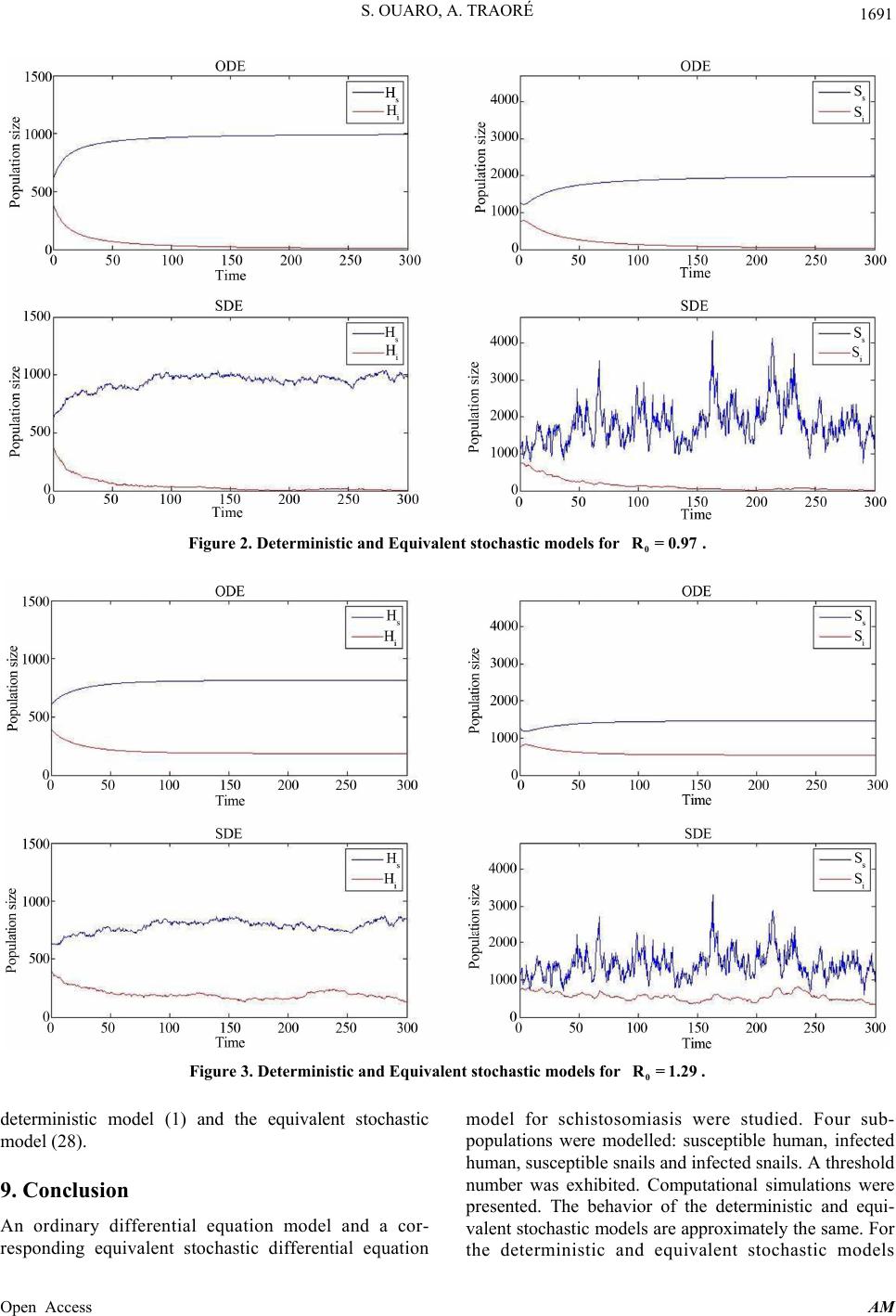

S. OUARO, A. TRAORÉ 1691
stic models for . Figure 2. Deterministic an
0
R= 0.97 d Equivalent stocha
Figure 3. Deterministic and Equivalent stochastic models for
deterministic model (1) and the equivalent stochastic
model (28).
9. Conclusion
An ordinary differential equation model and a cor-
responding equivalent stochastic differential equation
model for schistosomiasis were studied. Four sub-
populations were modelled: susceptible human, infected
human, susceptible snails and infected snails. A threshold
number was exhibited. Computational simulations were
presented. The behavior of the deterministic and equi-
valent stochastic models are approximately the same. For
the deterministic and equivalent stochastic models
0
R= 1.29 .
Open Access AM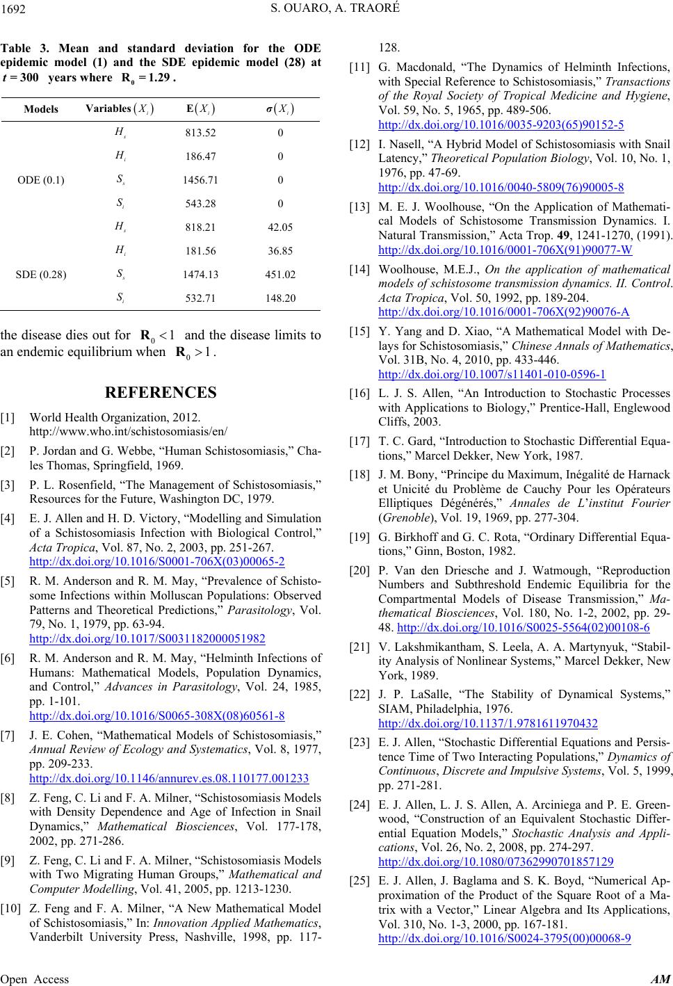

S. OUARO, A. TRAORÉ
1692
Table 3. Mean and standard deviation for the ODE
epidemic model (1) and the SDE epidemic model (28) at
years where
Models Variables
t=300 0 R= 1.29 .

i
X

i
XE


i
Xσ
s
H
813.52 0
i
H
186.47 0
ODE (0.1)
s
S 1456.71 0
543.28 0
i
S
s
H
818.21 42.05
i
H
181.56 36.85
SDE (0.28)
s
S 1474.13 451.02
532.71 148.20
i
S
the disease dies out for and the disease limits to
an endemic equilibrium
REFERENCES
[1] World Health Organization, 2012.
http://www.who.int/schistosomiasis/en/
P. Jordan and G. Webbe, “Hum
les Thomas, Springfield, 1969.
[3] P. L. Rosenfield, “The Management of Schistosomiasis,”
Resources for the Future, Washington DC, 1979.
[4] E. J. Allen and H. D. Victory, “Modelling and Simulation
of a Schistosomiasis Infection with Biological Control,”
Acta Tropica, Vol. 87, No. 2, 2003, pp. 251-267.
http://dx.doi.org/10.1016/S0001-706X(03)00065-2
01R
when R01.
[2] an Schistosomiasis,” Cha-
[5] R. M. Anderson and R. M. May, “Prevalence of Schisto-
some Infections within Molluscan Populations: Observed
Patterns and Theoretical Predictions,” Parasitology, Vol.
79, No. 1, 1979, pp. 63-94.
http://dx.doi.org/10.1017/S0031182000051982
[6] R. M. Anderson and R. M. May, “Helminth Infections of
Humans: Mathematical Models, Population Dynamics,
and Control,” Advances in Parasitology, Vol. 24, 1985,
pp. 1-101.
http://dx.doi.org/10.1016/S0065-308X(08)60561-8
[7] J. E. Cohen, “Mathematical Models of Schistosomiasis,”
Annual Review of Ecology and Systematics, Vol. 8, 1977,
pp. 209-233.
http://dx.doi.org/10.1146/annurev.es.08.110177.001233
[8] Z. Feng, C. Li and F. A. Milner, “Schistosomiasis Models
with Density Dependence and Age of Infection in Snail
Dynamics,” Mathemati
2002, pp. 271-286.
] Z. Feng, C. Li and F. A. Milner, “Schistosomiasis Models
r Modelling, Vol. 41, 2005, pp. 1213-1230.
[10] Z. Feng and F. A. Milner, “A New Mathematical Model
asis,” In: Innovation Applied Mathematics,
iversity Press, Nashville, 1998, pp. 117-
128.
[11] G. Macdonald, “The Dynamics of Helminth Infections,
with Special Reference to Schistosomiasis,” Transactions
of the Royal Society of Tropical Medicine and Hygiene,
Vol. 59, No. 5, 1965, pp. 489-506.
http://dx.doi.org/10.1016/0035-9203(65)90152-5
[12] I. Nasell, “A Hybrid Model of Schistosomiasis with Snail
Latency,” Theoretical Population Biology, Vol. 10, No. 1,
1976, pp. 47-69.
http://dx.doi.org/10.1016/0040-5809(76)90005-8
[13] M. E. J. Woolhouse, “On the Application of Mathemati-
cal Models of Schistosome Transmission Dynamics. I.
Natural Tra nsmission,” Acta Trop. 49, 1241-1270, (1991).
http://dx.doi.org/10.1016/0001-706X(91)90077-W
[14] Woolhouse, M.E.J., On the application of mathematical
models of schistosome transmission dynamics. II. Control.
Acta Tropica, Vol. 50, 1992, pp. 189-204.
http://dx.doi.org/10.1016/0001-706X(92)90076-A
[15] Y. Yang and D. Xiao, “A Mathematical Model with De-
lays for Schistosomiasis,” Chinese Annals of Mathematics,
Vol. 31B, No. 4, 2010, pp. 433-446.
http://dx.doi.org/10.1007/s11401-010-0596-1
[16] L. J. S. Allen, “An Introduction to Stochastic Processes
with Applications to Biology,” Prentice-Hall, Englewood
Cliffs, 2003.
duction to Stochastic Differential Equa-
tions,” Marcel Dekker, New York, 1987.
[18] J. M. Bony, “Principe du Maximum, Inégalité de Harnack
et Unicité du Problème de Cauchy Pour les Opérateurs
Elliptiques Dégénérés,” Annales de L’institut Fourier
(Grenoble), Vol. 19, 1969, pp. 277-304.
[19] G. Birkhoff and G. C. Rota, “Ordinary Differential Equa-
tions,” Ginn, Boston, 1982.
[20] P. Van den Driesche and J. Watmough, “Reproduction
Numbers and Subthreshold Endemic Equilibria for the
Compartmental Models of Disease Transmission,” Ma-
thematical Biosciences, Vol. 180, No. 1-2, 2002, pp. 29-
48. http://dx.doi.org/10.1016/S0025-5564(02)00108-6
cal Biosciences, Vol. 177-178,
[9 with Two Migrating Human Groups,” Mathematical and
Compute
of Schistosomi
Vanderbilt Un
[17] T. C. Gard, “Intro
[21] V. Lakshmikantham, S. Leela, A. A. Martynyuk, “Stabil-
ity Analysis of Nonlinear Systems,” Marcel Dekker, New
York, 1989.
[22] J. P. LaSalle, “The Stability of Dynamical Systems,”
SIAM, Philadelphia, 1976.
http://dx.doi.org/10.1137/1.9781611970432
[23] E. J. Allen, “Stochastic Differential Equations and Persis-
tence Time of Two Interacting Populations,” Dynamics of
Continuous, Discrete and Impulsive Systems, Vol. 5, 1999,
pp. 271-281.
[24] E. J. Allen, L. J. S. Allen, A. Arciniega and P. E. Green
wood, “Construction of an Equivalent Stochastic Diffe
odels,” Ststic Analysis and Appli-
, 2008. 274-297.
-
r-
ential Equation Mocha
cations, Vol. 26, No. 2, pp
http://dx.doi.org/10.1080/07362990701857129
[25] E. J. Allen, J. Baglama and S. K. Boyd, “Numerical Ap-
proximation of the Product of the Square Root of a Ma-
trix with a Vector,” Linear Algebra and Its Applications,
Vol. 310, No. 1-3, 2000, pp. 167-181.
http://dx.doi.org/10.1016/S0024-3795(00)00068-9
Open Access AM

S. OUARO, A. TRAORÉ
Open Access AM
1693
[26] Z. Feng, A. Eppert, F. A. Milner and D. J. Minchella,
“Estimation of Paramaters Governing the Transmission
Dynamics of Schistosomes,” Applied Mathematics Let-
ters, Vol. 17, No. 10, 2004, pp. 1105-1112.
http://dx.doi.org/10.1016/j.aml.2004.02.002