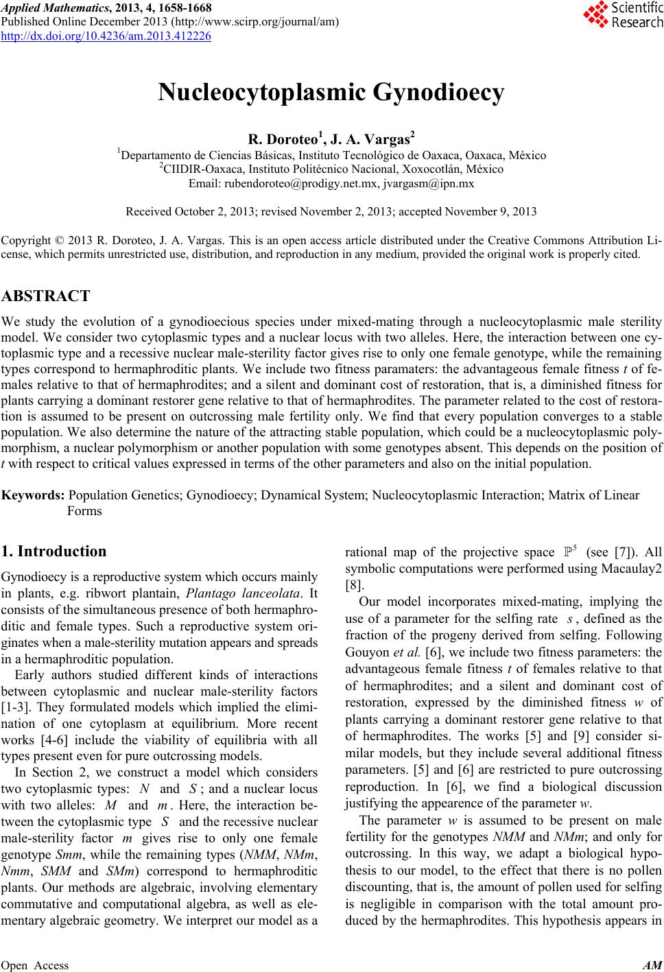
 Applied Mathematics, 2013, 4, 1658-1668 Published Online December 2013 (http://www.scirp.org/journal/am) http://dx.doi.org/10.4236/am.2013.412226 Open Access AM Nucleocytoplasmic Gynodioecy R. Doroteo1, J. A. Vargas2 1Departamento de Ciencias Básicas, Instituto Tecnológico de Oaxaca, Oaxaca, México 2CIIDIR-Oaxaca, Instituto Politécnico Nacional, Xoxocotlán, México Email: rubendoroteo@prodigy.net.mx, jvargasm@ipn.mx Received October 2, 2013; revised November 2, 2013; accepted November 9, 2013 Copyright © 2013 R. Doroteo, J. A. Vargas. This is an open access article distributed under the Creative Commons Attribution Li- cense, which permits unrestricted use, distribution, and reproduction in any medium, provided the original work is properly cited. ABSTRACT We study the evolution of a gynodioecious species under mixed-mating through a nucleocytoplasmic male sterility model. We consider two cytoplasmic types and a nuclear locus with two alleles. Here, the interaction between one cy- toplasmic type and a recessive nuclear male-sterility factor gives rise to only one female genotype, while the remaining types correspond to hermaphroditic plants. We include two fitness paramaters: the advantageous female fitness t of fe- males relative to that of hermaphrodites; and a silent and dominant cost of restoration, that is, a diminished fitness for plants carrying a dominant restorer gene relative to that of hermaphrodites. The parameter related to the cost of restora- tion is assumed to be present on outcrossing male fertility only. We find that every population converges to a stable population. We also determine the nature of the attracting stable population, which could be a nucleocytoplasmic poly- morphism, a nuclear polymorphism or another population with some genotypes absent. This depends on the position of t with respect to critical values expressed in terms of the other parameters and also on the initial population. Keywords: Population Genetics; Gynodioecy; Dynamical System; Nucleocytoplasmic Interaction; Matrix of Linear Forms 1. Introduction Gynodioecy is a reproductive system which occurs mainly in plants, e.g. ribwort plantain, Plantago lanceolata. It consists of the simultaneous presence of both hermaphro- ditic and female types. Such a reproductive system ori- ginates when a male-sterility mutation appears and spreads in a hermaphroditic population. Early authors studied different kinds of interactions between cytoplasmic and nuclear male-sterility factors [1-3]. They formulated models which implied the elimi- nation of one cytoplasm at equilibrium. More recent works [4-6] include the viability of equilibria with all types present even for pure outcrossing models. In Section 2, we construct a model which considers two cytoplasmic types: and ; and a nuclear locus with two alleles: N S and m. Here, the interaction be- tween the cytoplasmic type and the recessive nuclear male-sterility factor gives rise to only one female genotype Smm, while the remaining types (NMM, NMm, Nmm, SMM and SMm) correspond to hermaphroditic plants. Our methods are algebraic, involving elementary commutative and computational algebra, as well as ele- mentary algebraic geometry. We interpret our model as a rational map of the projective space (see [7]). All symbolic computations were performed using Macaulay2 [8]. S m 5 Our model incorporates mixed-mating, implying the use of a parameter for the selfing rate , defined as the fraction of the progeny derived from selfing. Following Gouyon et al. [6], we include two fitness parameters: the advantageous female fitness t of females relative to that of hermaphrodites; and a silent and dominant cost of restoration, expressed by the diminished fitness w of plants carrying a dominant restorer gene relative to that of hermaphrodites. The works [5] and [9] consider si- milar models, but they include several additional fitness parameters. [5] and [6] are restricted to pure outcrossing reproduction. In [6], we find a biological discussion justifying the appearence of the parameter w. The parameter w is assumed to be present on male fertility for the genotypes NMM and NMm; and only for outcrossing. In this way, we adapt a biological hypo- thesis to our model, to the effect that there is no pollen discounting, that is, the amount of pollen used for selfing is negligible in comparison with the total amount pro- duced by the hermaphrodites. This hypothesis appears in 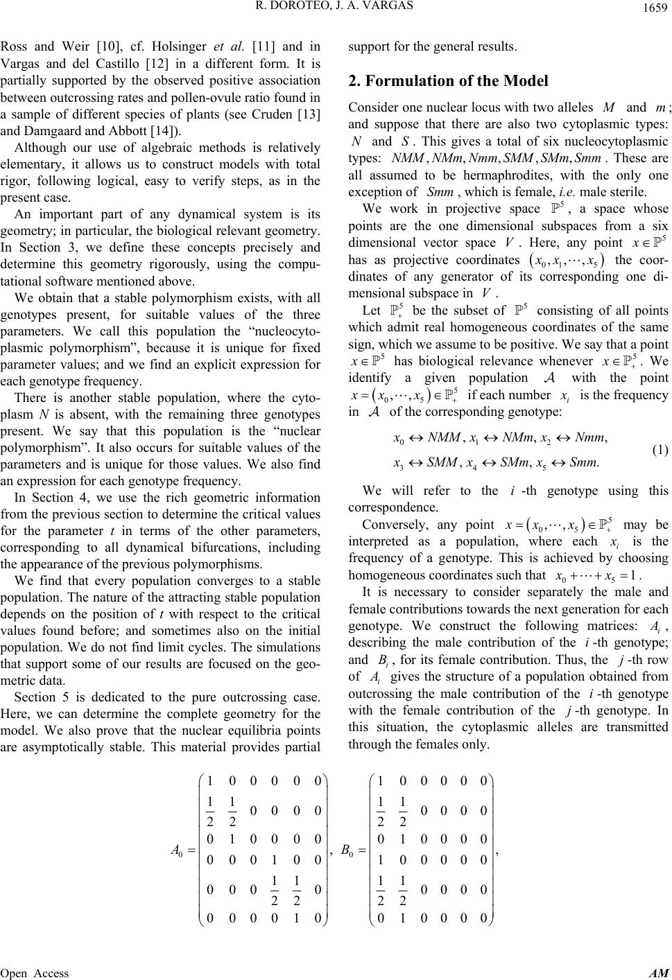 R. DOROTEO, J. A. VARGAS 1659 Ross and Weir [10], cf. Holsinger et al. [11] and in Vargas and del Castillo [12] in a different form. It is partially supported by the observed positive association between outcrossing rates and pollen-ovule ratio found in a sample of different species of plants (see Cruden [13] and Damgaard and Abbott [14]). Although our use of algebraic methods is relatively elementary, it allows us to construct models with total rigor, following logical, easy to verify steps, as in the present case. An important part of any dynamical system is its geometry; in particular, the biological relevant geometry. In Section 3, we define these concepts precisely and determine this geometry rigorously, using the compu- tational software mentioned above. We obtain that a stable polymorphism exists, with all genotypes present, for suitable values of the three parameters. We call this population the “nucleocyto- plasmic polymorphism”, because it is unique for fixed parameter values; and we find an explicit expression for each genotype frequency. There is another stable population, where the cyto- plasm N is absent, with the remaining three genotypes present. We say that this population is the “nuclear polymorphism”. It also occurs for suitable values of the parameters and is unique for those values. We also find an expression for each genotype frequency. In Section 4, we use the rich geometric information from the previous section to determine the critical values for the parameter t in terms of the other parameters, corresponding to all dynamical bifurcations, including the appearance of the previous polymorphisms. We find that every population converges to a stable population. The nature of the attracting stable population depends on the position of t with respect to the critical values found before; and sometimes also on the initial population. We do not find limit cycles. The simulations that support some of our results are focused on the geo- metric data. Section 5 is dedicated to the pure outcrossing case. Here, we can determine the complete geometry for the model. We also prove that the nuclear equilibria points are asymptotically stable. This material provides partial support for the general results. 2. Formulation of the Model Consider one nuclear locus with two alleles and ; and suppose that there are also two cytoplasmic types: and . This gives a total of six nucleocytoplasmic types: . These are all assumed to be hermaphrodites, with the only one exception of , which is female, i.e. male sterile. m N S NM ,,,,,MNMm Nmm SMMSMmSm Smm 5 m We work in projective space , a space whose points are the one dimensional subspaces from a six dimensional vector space V. Here, any point 5 x has as projective coordinates 01 5 ,, , xx the coor- dinates of any generator of its corresponding one di- mensional subspace in . V Let 5 be the subset of consisting of all points which admit real homogeneous coordinates of the same sign, which we assume to be positive. We say that a point 5 5 x has biological relevance whenever . We identify a given population with the point 5 x 5 05 x,,xx if each number i is the frequency in of the corresponding genotype: 012 345 ,, ,, , . NMMxNMm xNmm SMMxSMm xSmm (1) We will refer to the i-th genotype using this correspondence. Conversely, any point 5 05 ,,xx x may be interpreted as a population, where each i is the frequency of a genotype. This is achieved by choosing homogeneous coordinates such that . 05 It is necessary to consider separately the male and female contributions towards the next generation for each genotype. We construct the following matrices: i 1xx , describing the male contribution of the -th genotype; and i, for its female contribution. Thus, the -th row of i i Bj gives the structure of a population obtained from outcrossing the male contribution of the -th genotype with the female contribution of the -th genotype. In this situation, the cytoplasmic alleles are transmitted through the females only. i j 00 1 000 001 00000 11 11 00 000000 22 22 010000 010000 ,, 000100 100000 11 11 0 0000000 22 22 0 000 100 10000 AB Open Access AM 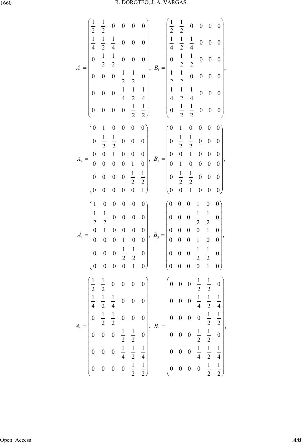 R. DOROTEO, J. A. VARGAS 1660 11 11 11 0000 0000 22 22 111 111 0 0 0000 424 424 11 11 00 0 00000 22 22 ,, 11 11 0 0 000000 22 22 111 111 0 0 0000 424 424 11 11 00000 000 22 22 AB 22 010000 010000 11 11 0000000 22 22 001000 001000 ,, 000010 010000 11 11 00000 000 22 22 000001 001000 AB 0 33 100000 000100 11 11 0000 0000 2222 010000 000010 ,, 0 001 000001 00 11 11 000 0000 0 22 22 000010 000010 AB 44 11 11 0000 0000 22 22 111 111 000 000 424 424 11 11 0000 0000 22 22 ,, 11 11 0000 0000 22 22 111 111 000 000 424 424 11 11 0000 0000 22 22 AB Open Access AM  R. DOROTEO, J. A. VARGAS Open Access AM 1661 55 01 000 000001 0 11 11 000 00000 22 22 00 100 000000 1 ,. 00 001 000001 0 11 11 00 000000 22 22 00 000 100000 1 AB Finally, we obtain the mixed-mating matrix 1TshS sQ, where 0 To compensate for its male sterility, the genotype has associated an enhanced female fertility, so that Smm female fertility of1. female fertility ofhermaphrodites Smm t 1 is the selfing rate; and 05 hx x is a homogenizing factor, first introduced by Holgate [15], it equals one in any biological context. The evolution map is , given by 55 : We assume that selection acts against plants that carry a dominant restorer gene together with the cytoplasm . Thus, the genotypes and have associated a diminished male fertility, so that NNMM NMm 05 ,, , xT yy (3) for 5 x . It provides the genotype frequencies for the next generation of any population . 5 x outcrossing male fertility of,1. outcrossing male fertility of hermaphrodites NMM NMm w 3. Geometry of the Dynamical System The parameter t is introduced through the female fitness matrix , while the male sterility and are introduced through the male fitness matrix . w G 100000 00000 0100000 0000 0010000 01000 , 0001000 00100 0000100 00010 000000 00000 w w FG t . We call trajectory any sequence 5 0,1, 2, i zi such that 1i z i , for all i. We start with the elementary observation that in case there is a trajectory 012 such that li , then the point must be a fixed point for the map, i.e. a point with z ,,,zzzmii zw w w w , or else it must be a fundamental point, i.e. a point where w is not defined because all its homogeneous coordinates would vanish. We say that the fixed point is stable whenever given a neighborhood v of , in the classical topology, we can find a neighborhood of such that all points in are sent to v v by n , for sufficiently large. We say that the fixed point is asymptotically stable, when, in addition to the above condition, there exists an open set , such that n v n n lim v for all . These definitions are adapted from those usually given for dynamical systems, see Hirsch and Smale [16]. x The evolution of this reproductive system has to be formulated using all possible crosses between genotypes. We first construct the outcrossing matrix as fol- lows: Q 00011 222 333 444 555 12 0. QxwFAGBx wFAGB xFAGBxFA GB xFAGBxFA tGB 1 (2) We will determine the geometry of the fixed and fundamental points of biological interest. If 1,, n f are homogeneous polynomials, we write their locus We next construct the selfing matrix , writing as its -th row half the sum of the -th row of the matrix i S i i with the -th row of i, for , except that the last row must be zero. Thus, iB 0i55 ,,Zffpf pfp 11nn 0 100000 14 12 14000 001000 . 000100 000141214 000000 S ; and similarly for infinite collections of homogeneous polynomials. If a is a homogeneous ideal of the polynomial ring 05 ,, x , is the locus of all of the homogeneous elements of . Za a Proposition 1. All fixed and fundamental points of biological interest for the map are among the following: 1) Those on the line , which consists of fixed points, except for the fundamental point 1245 ,,,L Zxxxx  R. DOROTEO, J. A. VARGAS 1662 5 1, 0,0,, 0,0fswsw a 0,0,1,b . 2) The fundamental point . 0, 0,0, 0,0,1 0,0,0 3) The fixed point . 4) The fixed point , 0,11ts0, 0,,0cs , provided 1 >1 t . 5) The pair of fixed points associated to the ideal 0 ,,, ,WRstwx x 5 generated by the following five forms: 103 214 325 2 10111201 0212 201 2 1, 1, 1, 4, 1 11 . pwxx pwxx pwxtx qtxxtxtxxxxx xxx qtstswst xx tst tswx (4) 6) The pair of fixed points associated to the ideal generated by the following forms: NR 012 3455 34 2 3435 44534 ,,, 122 42 xxx , . tx xxsxx x txxxx xxxxx (5) Proof 1. (1 - 4): The fixed and fundamental points of are associated to the ideal generated by the minors from the matrix whose rows are 2226 and . It is easy to verify that the points and and the line satisfy ,ab cL . It is equally easy to verify that among all these points, exactly the points and a are fundamental. (5 - 6): The ideal is difficult to handle. However, the ideals W and are easier to manage and they contain substantial information about fixed points of biological interest. The ideal 05 N ,, y of funda- mental points, is also easy to handle and it does not produce any further points of biological relevance. By Bézout’s theorem applied to the plane with homogeneous coordinates 012 2 ,, xx, we obtain that describes a pair of points, which are the intersection of a line and a conic. W Similarly, we see that describes a pair of points, by Bézout’s theorem applied to the plane with homogeneous coordinates N 345 ,, xx. We calculate the transporter :,WIz RzIW obtaining as a result an ideal containing the nonzero parameter . This means that the points corresponding to are fixed or fundamental points for our map. Then we saturate W with the ideal generated by , the coordinates of t 5 y W 0 ,,y . The result is . Thus, the points described by are fixed points of W W . An analogous process proves that the points described by are also fixed points. N Finally, we saturate the ideal with the ideal of fundamental points; then we saturate the result successively with and the ideals for the line , the points and . The result from the above process is an ideal whose primary decomposition shows no points of biological relevance. □ ,WN c L ,ab The fixed points in 5 05 ,, 05 0xx xxx correspond to polymorphisms with all genotypes present. Corollary 1. All fixed points in for the map are among those associated to the ideal . W Our immediate problem is to determine the nature of the pairs of points associated to and . First, we fix the notation. Let W N 1,2 22 1, 2 121 , 1 1141 1, 21 11 , 1 21 2122 45 sw sw ss w s sw s . wsssw sw ws (6) Lemma 1. These quantities satisfy: 11 0<<<< , where the last inequality requires 5sw<4 . 1 11<< <21 s . 12 < if and only if 4 . 5<sw ,<0 22 . Proof 2. We prove only the first assertion. The remaining assertions admit analogous proofs. The inequality 0< is clear. Since both numerators and denominators involved are positive, we verify that 1 < as follows: Since 1 2 11 2 2 2 21 11 141 11121 121 , 41 111 141141121 141121, sw s ss wsws sw ssws ws swss w swssw we have Open Access AM  R. DOROTEO, J. A. VARGAS 1663 2 11 2 2 2 3 41 111 11411 211 211 41 120. ssw s sws sw sswsw ssw w Here, we observe that 11 11<<s . We verify that 1< as follows: Since 1 211 2 11411, swss w it suffices to see that 2 2 121141 1 42 10. wss sww w We verify that 1 < provided as follows: Since both numerators and denominators involved are positive and 5<sw4 1 22 145 211 2211 451 21, ssw ssswsws w sws sw it suffices to see that 222 2 2 3 411 22 114 5121 45120. sssswsw sws wssw ssw ww One fixed point , described by W, has homo- geneous coordinates v 2 0 2 1 2 30415 2 211321 411521, 21 11, 1,1,1 . vttstw tww vttstwtwwB vtswts vwvvwvvwtv ,B (7) where 2 32 1181 19 111513. Bstwtt stwtw wtw One fixed point , satisfying , has homogeneous coordinates uN 012 3 2 4 5 0, 11 , 12 12. uuu utsts D ustsstt ust where 2 22 21212 2. Dtt s sts ttsstst The point has biological relevance exactly when the inequality u 1>st2 holds. The other point satisfying never has biological meaning. N The ideal corresponds to a pair of fixed points, one of which describes the associated nuclear poly- morphism, i.e . where exactly the genotypes are present. N ,SMM 5 ,SMm Smm Proposition 2. We have if and only if vv if and only if 1<<t . Proof We first observe that 2 2 21 211321 1. ttst wtwwB swttt Hence, if and only if 0>0v<t or 1 >t . We observe that 121 vtt B and also 2 21 21 1Bttst tt >0v1<<t . Hence, if and only if 1 21vts t . We finally observe that . Hence for 2 2>0v<t . We have verified that 1<<t implies 012 >0, >0,>0.vvv This clearly also implies 345 >0, >0,>0.vvv Thus, v if 1<<t . The reciprocal also follows from the above calculations, as well as the remaining equivalence involving . □ 5 Multiple simulations, both algebraic and graphic strongly suggest that the second point satisfying W never has biological meaning. Thus, we have nearly complete understanding of the biologically relevant geometry for our rational map . We state this information in biological terms: Proposition 3. The populations in equilibrium for our gynodioecy model are the following: 1) The nucleocytoplasmic polymorphism corre- sponding to the point with coordinates given by Equations (7). This is possible if and only if the parameters satisfy 1<<.t 2) The nuclear polymorphism corresponding to the point with coordinates given by Equations (8). This is possible if and only if the parameters satisfy u 2 >. 1 t ,D (8) 3) The populations without the nuclear allele m Open Access AM 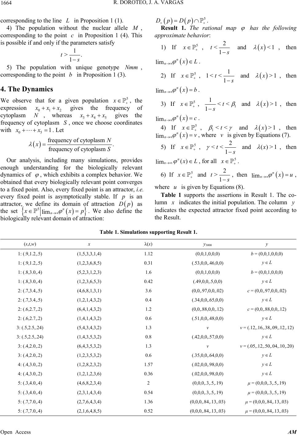 R. DOROTEO, J. A. VARGAS Open Access AM 1664 5 Dp Dp . corresponding to the line in Proposition 1 (1). LResult 1. The rational map has the following approximate behavior: 4) The population without the nuclear allele , corresponding to the point in Proposition 1 (4). This is possible if and only if the parameters satisfy c 1) If 5 x , 2 <1 t and , then <1x lim n n L . 1 >.t 1 5) The population with unique genotype , corresponding to the point in Proposition 1 (3). Nmm 2) If 5 x , 1 1< <1 t and , then >1x lim n n b . b 4. The Dynamics 3) If 5 x , 1 1<< 1t s and , then >1x n limn c . We observe that for a given population 5 x , the expression 201 xx N gives the frequency of cytoplasm , whereas 345 xx gives the frequency of cytoplasm , once we choose coordinates with . Let S5 4) If x , 1<<t and , then >1x lim n n v , where is given by Equations (7). v 0 x5 1x frequency of cytoplasm. frequency of cytoplasm N xS 5) If , 5 xs t1 2 << and 1>)(x , then , for all . Lx n)( n lim 5 x Our analysis, including many simulations, provides enough understanding for the biologically relevant dynamics of , which exhibits a complex behavior. We obtained that every biologically relevant point converges to a fixed point. Also, every fixed point is an attractor, i.e. every fixed point is asymptotically stable. If is an attractor, we define its domain of attraction p Dp as the set 6) If and 5 x2 >1 t , then lim n n u , where is given by Equations (8). u Table 1 supports the assertions in Result 1. The co- lumn indicates the initial population. The column indicates the expected attractor fixed point according to the Result. y 5lim n n xp . We also define the biologically relevant domain of attraction: Table 1. Simulations supporting Result 1. (s,t,w) x λ(x) y3000 y 1: (.9,1.2,.5) (1,5,3,3,1,4) 1.12 (0,0,1,0,0,0) b = (0,0,1,0,0,0) 1: (.9,1.2,.5) (1,2,3,6,8,5) 0.31 (.53,0,0,.46,0,0) yL 1: (.8,3.0,.4) (5,2,3,1,2,3) 1.6 (0,0,1,0,0,0) b = (0,0,1,0,0,0) 1: (.8,3.0,.4) (1,2,3,6,5,3) 0.42 (.49,0,0,.5,0,0) yL 2: (.7,3.4,.5) (4,6,8,1,3,1) 3.6 (0,0,.97,0,0,.02) c = (0,0,.97,0,0,.02) 2: (.7,3.4,.5) (1,2,1,4,3,2) 0.4 (.34,0,0,.65,0,0) yL 2: (.6,2.7,.2) (6,4,1,4,3,2) 1.2 (0,0,.88,0,0,.12) c = (0,0,.88,0,0,.12) 2: (.6,2.7,.2) (1,4,1,4,3,2) 0.6 (.51,0,0,.48,0,0) yL 3: (.5,2.5,.24) (5,4,3,4,3,2) 1.3 v v = (.12,.16,.38,.09,.12,.12) 3: (.5,2.5,.24) (1,4,3,5,3,2) 0.8 (.42,0,0,.57,0,0) yL 3: (.4,2.0,.2) (6,4,3,5,3,2) 1.3 v v = (.05,.12,.50,.04,.10,.20) 3: (.4,2.0,.2) (1,2,3,5,3,2) 0.6 (.35,0,0,.64,0,0) yL 4: (.4,3.0,.2) (1,2,8,2,3,2) 1.57 (.02,0,0,.98,0,0) yL 4: (.4,3.0,.2) (1,2,1,2,3,6) 0.36 (.02,0,0,.98,0,0) yL 5: (.3,4.0,.4) (4,6,8,2,3,4) 2 (0,0,0,.3,.5,.19) μ = (0,0,0,.3,.5,.19) 5: (.3,4.0,.4) (2,3,1,4,3,4) 0.54 (0,0,0,.3,.5,.19) μ = (0,0,0,.3,.5,.19) 5: (.7,7.0,.4) (2,7,6,4,3,4) 1.36 (0,0,0,.84,.13,.03) μ = (0,0,0,.84,.13,.03) 5: (.7,7.0,.4) (2,1,6,4,8,5) 0.52 (0,0,0,.84,.13,.03) μ = (0,0,0,.84,.13,.03)  R. DOROTEO, J. A. VARGAS 1665 Remarks. For easy reference, we restate Result 1 in more biological terms: 1) If 2 1< <1 t , every population with <1x , converges to an equilibrium population without the nuclear allele . m 2) If 1 1< <1 t , every population with >1x , converges to an equilibrium population with unique genotype . Nmm 3) If 1 1<< 1t s , every population with >1x , converges to an equilibrium population without the nuclear allele . 4) If 1<<t , every population with >1x , converges to the nucleocytoplasmic polymorphism. 5) If 2 << 1 t , every population with >1x , converges to an equilibrium population without the nuclear allele . m 6) If 2 >1 t , every population converges to the nuclear polymorphism. Remarks. The equation 1x being linear, de- fines a hyperplane in . Regarding Result 1, it is con- venient to consider the half-spaces 5 5>1Hx x 1 and its opposite 5 Hx x 2. In terms of domains of attraction, this Result reads as follows: 1 1) If 1< <t , then nearly equals . zL Dz 5 2 H 2) If 1 1<< 1t s , then nearly equals . Db 5 1 H 3) If 1 1<< 1t s , then nearly equals . Dc 5 1 H 4) If 1<<t , then nearly equals . Dv 5 1 H 5) If 2 << 1 t , then nearly equals . zL Dz 5 6) If 2 >1 t , then nearly equals Du 5 . Result 2. We list several refinements to Result 1. 1) For 1 1< <1 t , we have: a) stretches towards a region around the line segment Db ab consisting of points such that 5 x <1x . b) Dz z LL stretches towards a region around the line consisting of points such that 5 x >1x . 2) For 1 1<< 1t s, we have: a) z LL stretches towards a region around the line consisting of points such that Dz 5 x >1x . b) Here, >1c always holds. However, for values of the parameters such that is close to one, c Dc stretches to a small region around consisting of points c 5 x <<t such that . <1x 3) For 1 , we have: a) z LL stretches towards a region around the line consisting of points such that Dz 5 x >1x . b) Dz z bL stretches towards a region around the point consisting of points such that 5 x >1x . c) Dz z cL stretches towards a region around the point consisting of points such that 5 x >1x . d) Depending on the values of the parameters, Dv stretches towards a region around the line segment av consisting of points 5 x such that . <1x Table 2 supports the assertions in Result 2. 5. The Case of Pure Outcrossing We obtain a model for this case setting the parameter 0s . 5.1. Geometry Here, the set of fundamental points of the map is an algebraic set . It is the union of two linear spaces of dimensions three and one, respectively: 124023 2, wxx xwx x x 34120254 11 ,2, , 22 xxxxxxtx x The point 124 023 0,0,0,0,12 ,Z wxxxwxxx0,a is the unique element of with biological relevance. The set of fixed points of has closure equal to an algebraic set which admits different descriptions according to the values of the parameter : t 1) 1t . Here, has four irreducible components: 1, a conic; 2 a curve of degree 3; and two lines 1 and 2. The curve 2 contains no points of biological relevance because its points satisfy the equations C L C L C 012 345 0, 0.xxx xxx Open Access AM 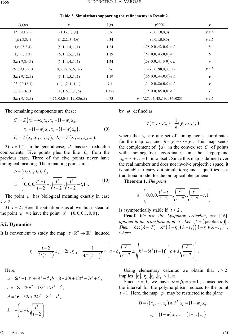 R. DOROTEO, J. A. VARGAS 1666 Table 2. Simulations supporting the refinements in Result 2. (s,t,w) x λ(x) y3000 y 1f: (.9,1.2,5) (1,1,6,1,1,8) 0.8 (0,0,1,0,0,0) yL 1f: (.8,3,4) (.1,2,2,.3,.4,6) 0.34 (0,0,1,0,0,0) yL 1g: (.8,3,4) (5,.1,.1,4,.1,.1) 1.24 .58, 0,0,.42, 0,0 b 1g: (.7,3,3) (6,.1,.1,5,.1,.1) 1.19 .57,0,0,.43,0,0 b 2a: (.7,3.4,3) (5,.1,.1,4,.1,.1) 1.24 .59, 0, 0,.41, 0,0 c 2b: (.9,10.2,.3) (0,0,.98,.5,.5,.02) 0.96 c = (0,0,.98,0,0,.02) yL 3a: (.9,12,.3) (6,.1,.1,5,.1,.1) 1.19 .56, 0, 0,.44, 0, 0 v 3b: (.9,16,3) (.1,.1,2,.1,.1,.1) 7.3 .14, 0, 0,.86, 0, 0 v 3c: (.9,16,3) (.1,.1,.9,.1,.1,.6) 1.375 .15, 0,0,.85,0, 0 v 3d: (.9,13,.3) (.27,.05,043,.19,.036,.8) 0.73 v = (.27,.05,.43,.19,.036,.023) yL The remaining components are these: 2 14355 2 4130 10134 21245 4, 1, 1,1 , ,,,, ,,, CZx xxxwx xwxxwx LZxxxxL Zxxxx . (9) 2) . In the general case, 1, 2t has six irreducible components: Five points plus the line 2 from the previous case. Three of the five points never have biological meaning. The remaining points are: L 233 0,0,1,0,0,0, 0, 0, 0,,,1. 222 b tt tt u ttt t 6 (10) The point has biological meaning exactly in case . u 2>t 3) . Here, the situation is as above, but instead of the point we have the point . 2t u 0,0,0,1,0,0u 5.2. Dynamics It is convenient to study the map induced 6 : by defined as 05 05 1 ,,,, , xyy h where the i are any set of homogeneous coordinates for the map y ; and 05 hy y . This map sends the complement of a in the convex set of points with nonnegative coordinates in the hyperplane 05 1xx into itself. Since this map is defined over the real numbers and does not involve projective space, it is suitable to carry out simulations; and it qualifies as a traditional model for the biological phenomena. Theorem 1. The point 233 0,0,0,, ,1 222 tt tt ut ttt is asymptotically stable if . >2t Proof. We use the Lyapunov criterion, see [16], applied to the transformation . Let jacobian u . Then 2 234 det rrrr 1 , where 33 2 22 1213,4 2 2 21 ,2,8 1 212 2 41 tt rrrr abkttcd ttt t tt . t Here, 2345 23 2345 234 3 6116 ,820187 82018 7, 16 32248, . 2 attttbtttt ctt ttt dtttt t kab t Using elementary calculus we obtain that implies >2t 1234 ,,, <rrrr 1. □ 4 , Since 0s , we have 11 ; consequently the interval for the polymorphism reduces to the point 1t . Here, the map may be restricted to the plane 5 05 3 415 ,,1 , 1,1 Dx xxwx 0 2 wx xwx . Open Access AM 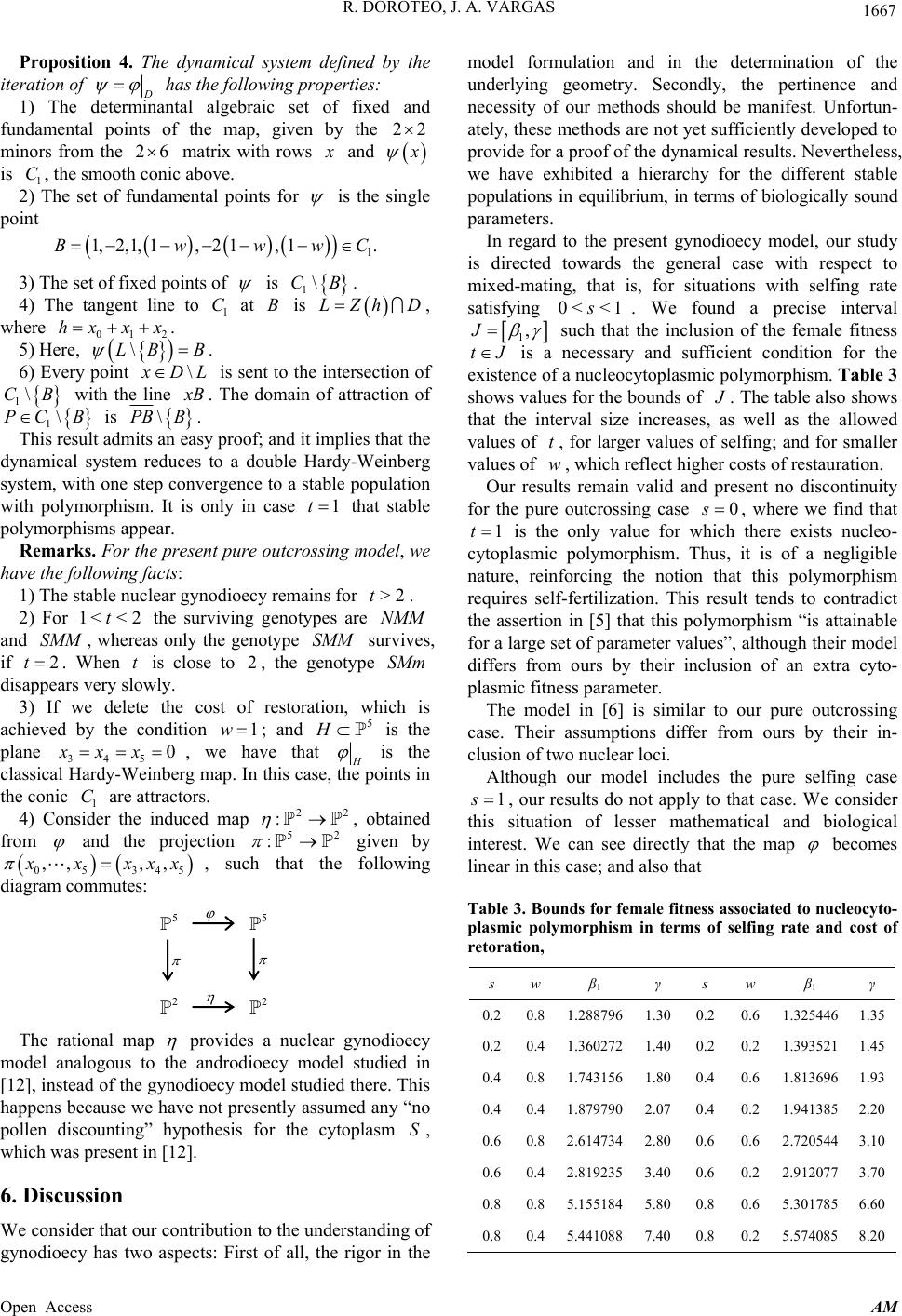 R. DOROTEO, J. A. VARGAS 1667 Proposition 4. The dynamical system defined by the iteration of has the following properties: 1) The determinantal algebraic set of fixed and fundamental points of the map, given by the 22 minors from the matrix with rows 26 and is , the smooth conic above. 1 2) The set of fundamental points for C is the single point 1 1,2,1, 1,2 1, 1.Bwww C 3) The set of fixed points of is . 1\CB 4) The tangent line to at is 1 CB h DLZ, where . 01 hxx x \LB 2 \ 5) Here, . B 6) Every point DL is sent to the intersection of with the line 1\CB B. The domain of attraction of is B 1\PC B\PB . This result admits an easy proof; and it implies that the dynamical system reduces to a double Hardy-Weinberg system, with one step convergence to a stable population with polymorphism. It is only in case that stable polymorphisms appear. 1t Remarks. For the present pure outcrossing model, we have the following facts: 1) The stable nuclear gynodioecy remains for . >2t 2) For the surviving genotypes are and , whereas only the genotype survives, if . When is close to , the genotype disappears very slowly. 1< <2t M t NMM SMm SM 2 SMM t2 3) If we delete the cost of restoration, which is achieved by the condition 1w ; and 5 is the plane 345, we have that 0xxx is the classical Hardy-Weinberg map. In this case, the points in the conic are attractors. 1 4) Consider the induced map , obtained from C 2 : 2 and the projection given by 5 345 52 : ,, 0 ,, xxxx , such that the following diagram commutes: 55 22 The rational map provides a nuclear gynodioecy model analogous to the androdioecy model studied in [12], instead of the gynodioecy model studied there. This happens because we have not presently assumed any “no pollen discounting” hypothesis for the cytoplasm , which was present in [12]. S 6. Discussion We consider that our contribution to the understanding of gynodioecy has two aspects: First of all, the rigor in the model formulation and in the determination of the underlying geometry. Secondly, the pertinence and necessity of our methods should be manifest. Unfortun- ately, these methods are not yet sufficiently developed to provide for a proof of the dynamical results. Nevertheless, we have exhibited a hierarchy for the different stable populations in equilibrium, in terms of biologically sound parameters. In regard to the present gynodioecy model, our study is directed towards the general case with respect to mixed-mating, that is, for situations with selfing rate satisfying . We found a precise interval 0< <1s 1,J tJ such that the inclusion of the female fitness is a necessary and sufficient condition for the existence of a nucleocytoplasmic polymorphism. Table 3 shows values for the bounds of . The table also shows that the interval size increases, as well as the allowed values of , for larger values of selfing; and for smaller values of , which reflect higher costs of restauration. t w Our results remain valid and present no discontinuity for the pure outcrossing case , where we find that 0s 1t is the only value for which there exists nucleo- cytoplasmic polymorphism. Thus, it is of a negligible nature, reinforcing the notion that this polymorphism requires self-fertilization. This result tends to contradict the assertion in [5] that this polymorphism “is attainable for a large set of parameter values”, although their model differs from ours by their inclusion of an extra cyto- plasmic fitness parameter. The model in [6] is similar to our pure outcrossing case. Their assumptions differ from ours by their in- clusion of two nuclear loci. Although our model includes the pure selfing case 1s , our results do not apply to that case. We consider this situation of lesser mathematical and biological interest. We can see directly that the map becomes linear in this case; and also that Table 3. Bounds for female fitness associate d to nucleocyto- plasmic polymorphism in terms of selfing rate and cost of retoration, s w β1 γ s w β1 γ 0.20.81.2887961.300.2 0.6 1.3254461.35 0.20.41.3602721.400.2 0.2 1.3935211.45 0.40.81.7431561.800.4 0.6 1.8136961.93 0.40.41.8797902.070.4 0.2 1.9413852.20 0.60.82.6147342.800.6 0.6 2.7205443.10 0.60.42.8192353.400.6 0.2 2.9120773.70 0.80.85.1551845.800.8 0.6 5.3017856.60 0.80.45.4410887.400.8 0.2 5.5740858.20 Open Access AM  R. DOROTEO, J. A. VARGAS Open Access AM 1668 114 023 ,0,,,0,0, lim 222 n n xxx xxxx [7] R. Hartshorne, “Algebraic Geometry,” In: Graduate Texts in Mathematics, Vol. 52, Springer, New York, 1977. [8] D. R. Grayson and M. E. Stillman, “Macaulay2, a Soft- ware System for Research in Algebraic Geometry.” http://www.math.uiuc.edu/Macaulay2 for any . If we assume that the cost of restoration is present in selfing, we obtain 5 x 14 23 0, 0,,, 0,0, lim 22 2 n n wx x xxx w [9] X. Delannay, P. H. Gouyon and G. Valdeyron, “Mathe- matical Study of the Evolution of Gynodioecy with Cyto- plasmic Inheritance under the Effect of a Nuclear Re- storer Gene,” Genetics, Vol. 99, 1981, pp. 169-181. http://www.ncbi.nlm.nih.gov/pmc/articles/PMC1214488/ for . 0< <1w [10] M. D. Ross and B. S. Weir, “Maintenance of Male Steril- ity in Plant Populations III. Mixed Selfing and Random Mating,” Heredity, Vol. 35, 1975, pp. 21-29. http://dx.doi.org/10.1038/hdy.1975.64 REFERENCES [1] E. Caspari, S. Watson and W. Smith, “The Influence of Cytoplasmic Pollen Sterility on Gene Exchange between Population,” Genetic s , Vol. 53, 1966, pp. 741-746. http://www.genetics.org/content/53/4/741.full.pdf [11] K. E. Holsinger, M. W. Feldman and F. B. Christiansen, “The Evolution of Self-Fertilization in Plants,” The Ame- rican Naturalist, Vol. 124, 1984, pp. 446-453. http://www.jstor.org/discover/10.2307/2461472?uid=373 8664uid=2129uid=2 uid=70 uid=4 sid=21102745754551 [2] D. Charlesworth and F.R. Ganders, “The Population Ge- netics of Gynodioecy with Cytoplasmic-Genic Male-Ste- rility,” Heredity, Vol. 43, 1979, pp. 213-218. http://dx.doi.org/10.1038/hdy.1979.76 [12] J. A. Vargas and R. F. del Castillo, “Nuclear Androdioecy and Gynodioecy,” Journal of Mathematical Biology, Vol. 47, No. 3, 2003, pp. 199-221. http://dx.doi.org/10.1007/s00285-003-0200-3 [3] G. S. Watson and E. Caspari, “The Behavior of Cytoplas- mic Pollen Sterility in Populations,” Evolution, Vol. 14, No. 1, 1960, pp. 56-63. http://dx.doi.org/10.2307/2405922 [13] R. W. Cruden, “Pollen-Ovule Ratios: A Conservative In- dicator of Breeding Systems in Flowering Plants,” Evolu- tion, Vol. 31, 1977, pp. 32-46. http://www.jstor.org/discover/10.2307/2407542?uid=373 8664uid=2129uid=2 uid=70 uid=4 sid=21102745773421 [4] M. F. Bailey, L. F. Delph and C. M. Lively, “Modelling Gynodioecy: Novel Scenarios for Maintaining Polymor- phism,” The American Naturalist, Vol. 161, No. 5, 2003, pp. 762-776. http://dx.doi.org/10.1086/374803 [14] C. Damgaard and R. J. Abbott, “Positive Correlations be- tween Selfing Rate and Pollen-Ovule Ratio within Plant Populations,” Evolution, Vol. 49, 1995, pp. 214-217. http://www.jstor.org/discover/10.2307/2410307?uid=373 8664uid=2129uid=2 uid=70 uid=4 sid=21102745773421 [5] M. Dufay, P. Touzet, S. Maurice and J. Cuguen, “Model- ling the Maintenance of Male-Fertile Cytoplasm in a Gynodioecious Population,” Heredity, Vol. 99, 2007, pp. 349-356. http://dx.doi.org/10.1038/sj.hdy.6801009 [15] P. Holgate, “Selfing in Genetic Algebras,” Journal of Ma- thematical Biology, Vol. 6, No. 2, 1978, pp. 197-206. http://dx.doi.org/10.1007/BF02450789 [6] P. H. Gouyon, F. Vichot and J. M. M. van Damme, “Nu- clear-Cytoplasmic Male Sterility: Single-Point Equilibria versus Limit Cycles,” The American Naturalist, Vol. 134, No. 4, 1991, pp. 498-513. http://www.jstor.org/discover/10.2307/2462377?uid=373 8664uid=2129 uid=2uid=70uid=4 sid=21102745687371 [16] M. Hirsch and S. Smale, “Differential Equations, Dyna- mical Systems and Linear Algebra,” Academic Press, New York, 1974.
|