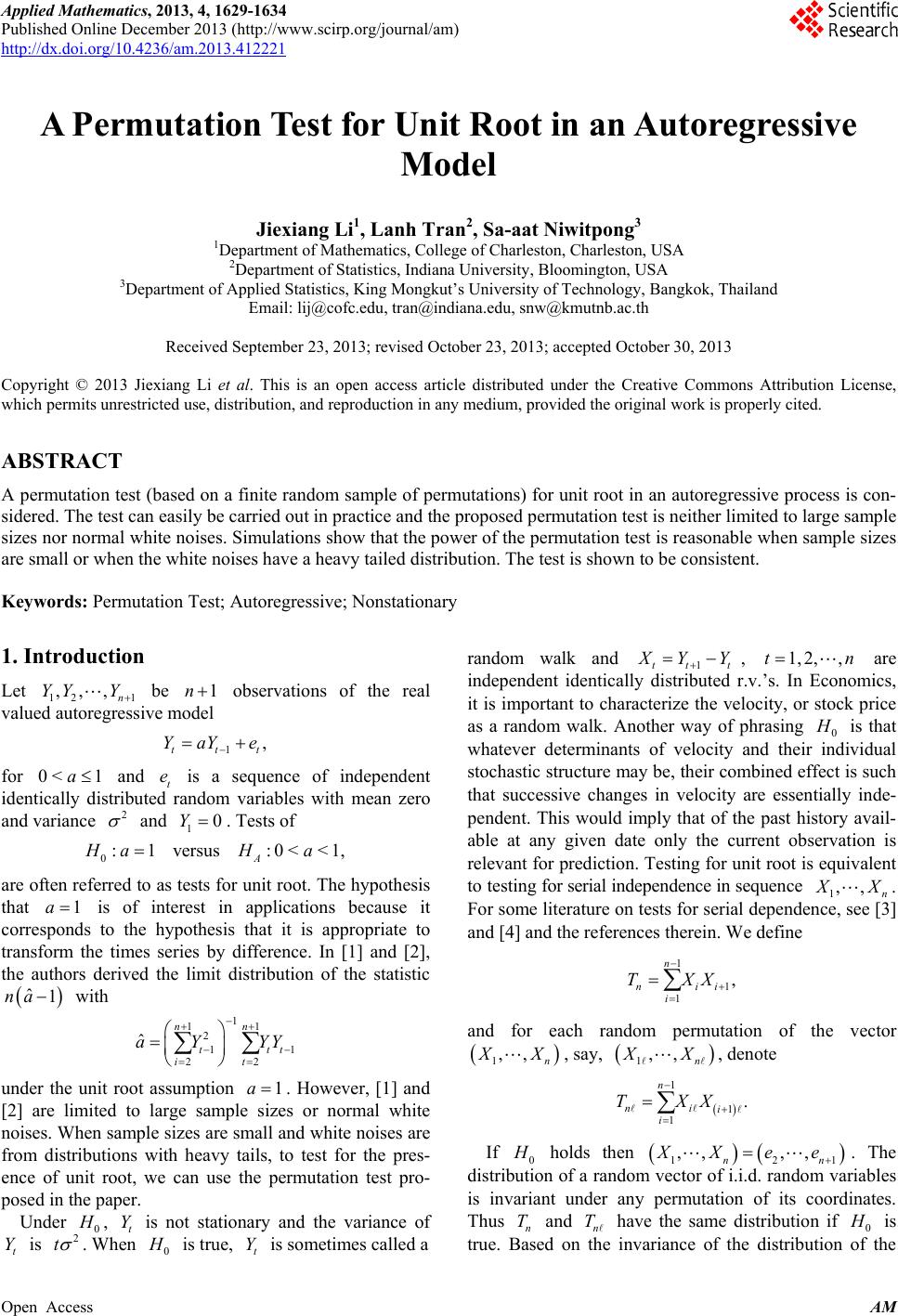
 Applied Mathematics, 2013, 4, 1629-1634 Published Online December 2013 (http://www.scirp.org/journal/am) http://dx.doi.org/10.4236/am.2013.412221 Open Access AM A Permutation Test for Unit Root in an Autoregressive Model Jiexiang Li1, Lanh Tran2, Sa-aat Niwitpong3 1Department of Mathematics, College of Charleston, Charleston, USA 2Department of Statistics, Indiana University, Bloomington, USA 3Department of Applied Statistics, King Mongkut’s University of Technology, Bangkok, Thailand Email: lij@cofc.edu, tran@indiana.edu, snw@kmutnb.ac.th Received September 23, 2013; revised October 23, 2013; accepted October 30, 2013 Copyright © 2013 Jiexiang Li et al. This is an open access article distributed under the Creative Commons Attribution License, which permits unrestricted use, distribution, and reproduction in any medium, provided the original work is properly cited. ABSTRACT A permutation test (based on a finite random sample of permutations) for unit root in an autoregressive process is con- sidered. The test can easily be carried out in practice and the proposed permutation test is neither limited to large sample sizes nor normal white noises. Simulations show that the power of the permutation test is reasonable when sample sizes are small or when the white noises have a heavy tailed distribution. The test is shown to be consistent. Keywords: Permutation Test; Autoregressive; Nonstationary 1. Introduction Let 12 1 be observations of the real valued autoregressive model ,,, n YY Y 1n 1, tt YaY e t for and t is a sequence of independent identically distributed random variables with mean zero and variance 0< 1ae 2 and . Tests of 10Y 0:1versus: 0<< 1, A HaH a are often referred to as tests for unit root. The hypothesis that is of interest in applications because it corresponds to the hypothesis that it is appropriate to transform the times series by difference. In [1] and [2], the authors derived the limit distribution of the statistic with 1a 1 ˆ na 1 11 2 11 22 ˆ nn tt it aY YY t under the unit root assumption . However, [1] and [2] are limited to large sample sizes or normal white noises. When sample sizes are small and white noises are from distributions with heavy tails, to test for the pres- ence of unit root, we can use the permutation test pro- posed in the paper. 1a Under 0 , t is not stationary and the variance of is tY t Y2 . When 0 is true, is sometimes called a t Y random walk and 1tt t YY , are independent identically distributed r.v.’s. In Economics, it is important to characterize the velocity, or stock price as a random walk. Another way of phrasing 0 1, 2,,tn is that whatever determinants of velocity and their individual stochastic structure may be, their combined effect is such that successive changes in velocity are essentially inde- pendent. This would imply that of the past history avail- able at any given date only the current observation is relevant for prediction. Testing for unit root is equivalent to testing for serial independence in sequence 1n ,, X. For some literature on tests for serial dependence, see [3] and [4] and the references therein. We define 1 1 1 , n nii i TXX and for each random permutation of the vector 1,, n X, say, 1,, n X , denote 1 1 1 . n ni i i TXX If 0 holds then 12 ,, ,, nn XXee 1 . The distribution of a random vector of i.i.d. random variables is invariant under any permutation of its coordinates. Thus n and n T have the same distribution if 0 T is true. Based on the invariance of the distribution of the  J. X. LI ET AL. 1630 statistic n under permutations when 0 T holds, we propose a permutation test for unit root using n as our pivot test statistic. This test is easy to perform with a computer and the test makes little assumptions on the probability distribution of the white noise and also it works for small samples. Construction of this test will be presented in Section 2. The consistency of our test is shown in Section 3. A simulation study of our test is provided in Section 4. Time series of velocity of money observed between 1869 and 1960 is investigated in Sec- tion 5. T 2. Steps Used in Our Permutation Test We assume that the white noise t e is a sequence of independent identically distributed random variables with mean zero and variance 2 . In addition, 4< t Ee . We will often write n T simply as for brevity. Note that T is more likely to be negative under A T (see Lemma 3.2 below). To summarize, the permutation test is carried out as follows. 1) Set a predetermined level . Permute the observations 12 n ,,, n XX. There are a total of permutations. For each permutation, compute the T statistic. Under 0 !n , the T statistics have the same probability distribution for all of the permutations. The statistic computed from the observations (not permuted) is referred to as . !n T obs 2) Compute the -value as the proportion of T's less than or equal to , that is, T p obs T numberof -value . obs T ! Ts pn Conclude that the test is statistically significant if the computed -value is less than or equal to p . This test is limited by prohibitive calculation and hard to carry out if is a large number. Instead of using all permutations to compute the , we obtain a random sample of permutations and then carry out the test as follows: n !n-valpue R 1) Set a predetermined level . Compute the T statistic for each of the sampled permutation. R 2) Compute the -value as the proportion of T's less than or equal to , that is, p obs T numberof -value . obs TTs pR Conclude that the test is statistically significant if the computed -value is less than or equal to p . The approximate -value is now equal to the fraction of 's that are less than or equal to obs . The theory of the binomial distribution tells us that the approximate value has about a 95% chance of being within p T T 21ppR of the true -value. We will denote the permutation test based on a random sample of permutations by pR . Remark. Consider the lag one autocorrelation 1 1 1 12 1 . n ii i n i i XXX rXX Using is “almost” equivalent to using 1 to perform our test. We leave it to the reader to verify this. Tr 3. Consistency of Consistency of hypothesis tests is a desirable property. In this section, we will show that the permutation test based on random sampling permutations is consistent, that is, the probability of correctly rejecting the null hypothe- sis R 0 tends to 1 as the sample size goes to infinity when . In other words, 0< <1a Theorem 3.1 Suppose a is an arbitrary simple hypothesis that the autoregressive parameter is between 0 and 1, that is a aA H. Then 0 Reject 1 a H PH as . n Lemma 3.1 Under A , for any integer , 1m 2 11 11 22. 1 mm m m EXXa aa a Proof. We can write as t Y 0 . u t u Yae t u (1) Using (1), it is easily seen that under A , the AR(1) process has mean zero with t Y 2 2 Var , 1 t Ya and 2 2. 1 m ttm EYY a a Clearly, 1122211211 . mmmm EXXEYYYY YYYY m In particular, 2 12 1, 1 a EXX a which is negative under A . Note Open Access AM  J. X. LI ET AL. 1631 22 12 11 2 2 0000 24412124224 1 00 01 222 44 424 2 2 4 24 2 2 2 11 1 1. 1 1 uv pq uvp q uvp q uuv u uuvuuvu t EYY Eae aeaeae aEe aaaa aaa Ee aa a a a a uv (2) Lemma 3.2 Under A , n Tn converges in proba- bility to 21 1 12 a EXX a Proof. Under A , time series is stationary and so is time series t Y 1tt X. Thus 12 , 1 n T EEX n X it suffices to show that Var 0. 1 n T n 121 1 11 1 1212 1 2 1212 23 12 34 12 12 112 4 Var 1Var2 Cov, 1Var2Cov , 1Var2 2Cov, 23Cov , 2. n iij j ijn n jj j n jj j T nXX XXXX nXXnjXXXX nXXnXXXX nXXXX njEXXXX EXX (3) By (3), it is sufficient to show that 2 1 12 112 4 20 1 n jj jnjEXXXX EXX n as . n For , consider . Following the proof of (2), we have 4j 12 1jj EXXXX 12 1 23 22 21 2 4 4 222123 4 4 234 4 2 2 23 2221 2 4 4 21 22 23 4 4 24 2322 212 4 2 2 332 1 33 1 14 64 1 3996 1 993 1 281282 . 1 jj jjjj t jjj t jjjj jjj jj jjj EXXXX aaaa Ee a aaa Ee a aa aa a aaaa a aaa a aa aaa a It is not hard to see that 123 22 21 2 2 4 12122 23 2 4 1332 1 133 1 n 0 jj j njjj j nj aaaa n nj aaa n j and 234 1 2 22 4 24 2322 212 1 2 22 4 2 1 22 4 14 64 11 281282 11 10 11 n j jjj n j n j aa aa nj na aaaaa nj na a njna j as . This completes the proof. n On the left of Figures 1 and 2, it shows the long run behavior of n Tn based on 10,000 simulations from AR(1) model with white noise from normal (0,1) and uniform (−1,1) respectively. Lemma 3.3 Under A , as . 12 0EXX n Proof. For a random permutation, R , of 12 ,, n. XX 12 1 1 ij PXX XXnn for any 1ijn . 1212 1 1 ,, 2. 1 n ij ijn EXXEEXXXX EXX nn (4) Open Access AM 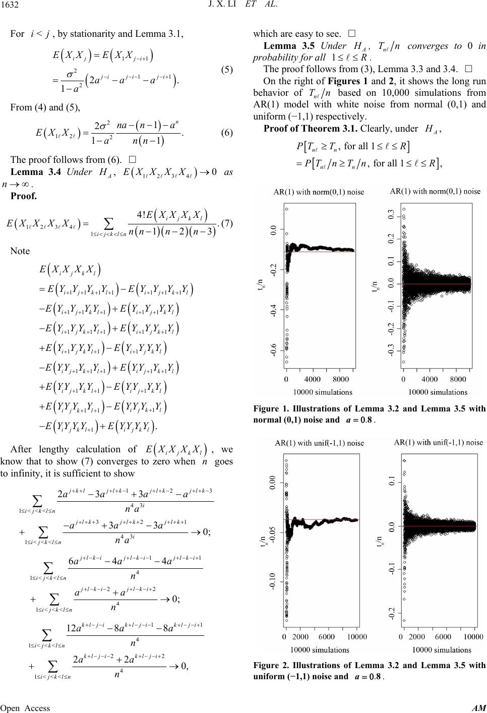 J. X. LI ET AL. 1632 For , by stationarity and Lemma 3.1, <ij 11 2 11 22. 1 ij ji ji jiji EXX EXX aa a a (5) From (4) and (5), 2 12 2 1 2. 1 1 n na na EXX nn a (6) The proof follows from (6). Lemma 3.4 Under A , as . 12340EXXXX n Proof. 1234 1 4! . 123 ijkl ijkln EXXXX EXXXXnn nn (7) Note 1111 111 11 111 111 11 11 1 111 11 11 1 11 ijkl ijkl ijkl ijkl ijkl ijkl ijkl ijkl ijkl ij k lij k l ij klij kl ijkl EXXXX EY YYYEY YYY EY YYYEY YYY EY YYYEY YYY EY YYYEY YYY EYYY YEYYY Y EYY YYEYY YY EYYYY 1 1. ijk l ijkl ijkl EYYYY EYYYYEYYYY After lengthy calculation of , we know that to show (7) converges to zero when goes to infinity, it is sufficient to show ijkl EXXXX n 12 43 1<<< 321 43 1<<< 23 3 33 0; jkl jlkjlkjlk i ijkln jlk jlk jlk i ijkln aaa a na aaa na 3 11 4 1<<< 22 4 1<<< 64 4 0; lkijlkijlki ijkln jlki jlki ijkln aa a n aa n 11 4 1<<< 22 4 1<<< 12 88 22 0, kl jikl jikl ji ijkln kljikl ji ijkln aa a n aa n which are easy to see. Lemma 3.5 Under A , n Tn converges to 0 in probability for all 1R . The proof follows from (3), Lemma 3.3 and 3.4. On the right of Figures 1 and 2, it shows the long run behavior of n Tn based on 10,000 simulations from AR(1) model with white noise from normal (0,1) and uniform (−1,1) respectively. Proof of Theorem 3.1. Clearly, under A , ,forall1 ,forall1 , nn nn PT TR PTnT nR Figure 1. Illustrations of Lemma 3.2 and Lemma 3.5 with normal (0,1) noise and .a8 . Figure 2. Illustrations of Lemma 3.2 and Lemma 3.5 with uniform (−1,1) noise and .a8 . Open Access AM 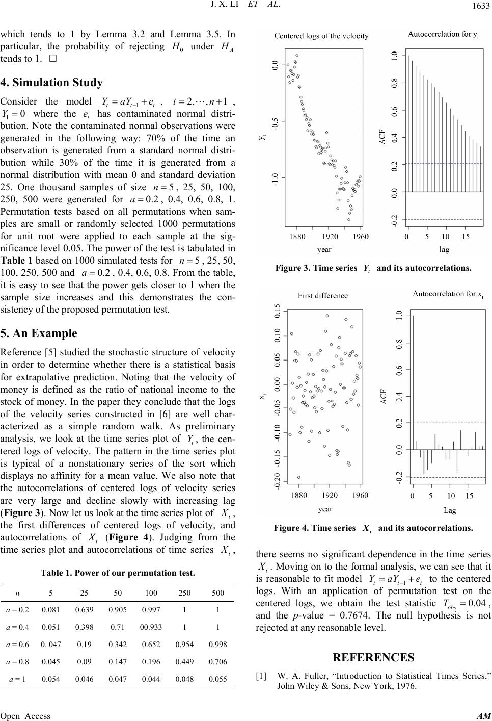 J. X. LI ET AL. 1633 which tends to 1 by Lemma 3.2 and Lemma 3.5. In particular, the probability of rejecting 0 under A tends to 1. 4. Simulation Study Consider the model 1ttt , , 1 where the t has contaminated normal distri- bution. Note the contaminated normal observations were generated in the following way: 70% of the time an observation is generated from a standard normal distri- bution while 30% of the time it is generated from a normal distribution with mean 0 and standard deviation 25. One thousand samples of size , 25, 50, 100, 250, 500 were generated for , 0.4, 0.6, 0.8, 1. Permutation tests based on all permutations when sam- ples are small or randomly selected 1000 permutations for unit root were applied to each sample at the sig- nificance level 0.05. The power of the test is tabulated in Table 1 based on 1000 simulated tests for , 25, 50, 100, 250, 500 and , 0.4, 0.6, 0.8. From the table, it is easy to see that the power gets closer to 1 when the sample size increases and this demonstrates the con- sistency of the proposed permutation test. YaY e n 0.2a 0.2 2, ,1tn 5 5n 0Ye a 5. An Example Reference [5] studied the stochastic structure of velocity in order to determine whether there is a statistical basis for extrapolative prediction. Noting that the velocity of money is defined as the ratio of national income to the stock of money. In the paper they conclude that the logs of the velocity series constructed in [6] are well char- acterized as a simple random walk. As preliminary analysis, we look at the time series plot of t, the cen- tered logs of velocity. The pattern in the time series plot is typical of a nonstationary series of the sort which displays no affinity for a mean value. We also note that the autocorrelations of centered logs of velocity series are very large and decline slowly with increasing lag (Figure 3). Now let us look at the time series plot of t Y , the first differences of centered logs of velocity, and autocorrelations of t (Figure 4). Judging from the time series plot and autocorrelations of time series t , Table 1. Power of our permutation test. n 5 25 50 100 250 500 a = 0.2 0.081 0.639 0.905 0.997 1 1 a = 0.4 0.051 0.398 0.71 00.933 1 1 a = 0.6 0. 047 0.19 0.3420.652 0.9540.998 a = 0.8 0.045 0.09 0.1470.196 0.4490.706 a = 1 0.054 0.046 0.047 0.044 0.048 0.055 Figure 3. Time series and its autocorrelations. t Y Figure 4. Time series t and its autocorrelations. there seems no significant dependence in the time series t . Moving on to the formal analysis, we can see that it is reasonable to fit model 1ttt to the centered logs. With an application of permutation test on the centered logs, we obtain the test statistic YaY e 0.04 obs T , and the p-value = 0.7674. The null hypothesis is not rejected at any reasonable level. REFERENCES [1] W. A. Fuller, “Introduction to Statistical Times Series,” John Wiley & Sons, New York, 1976. Open Access AM 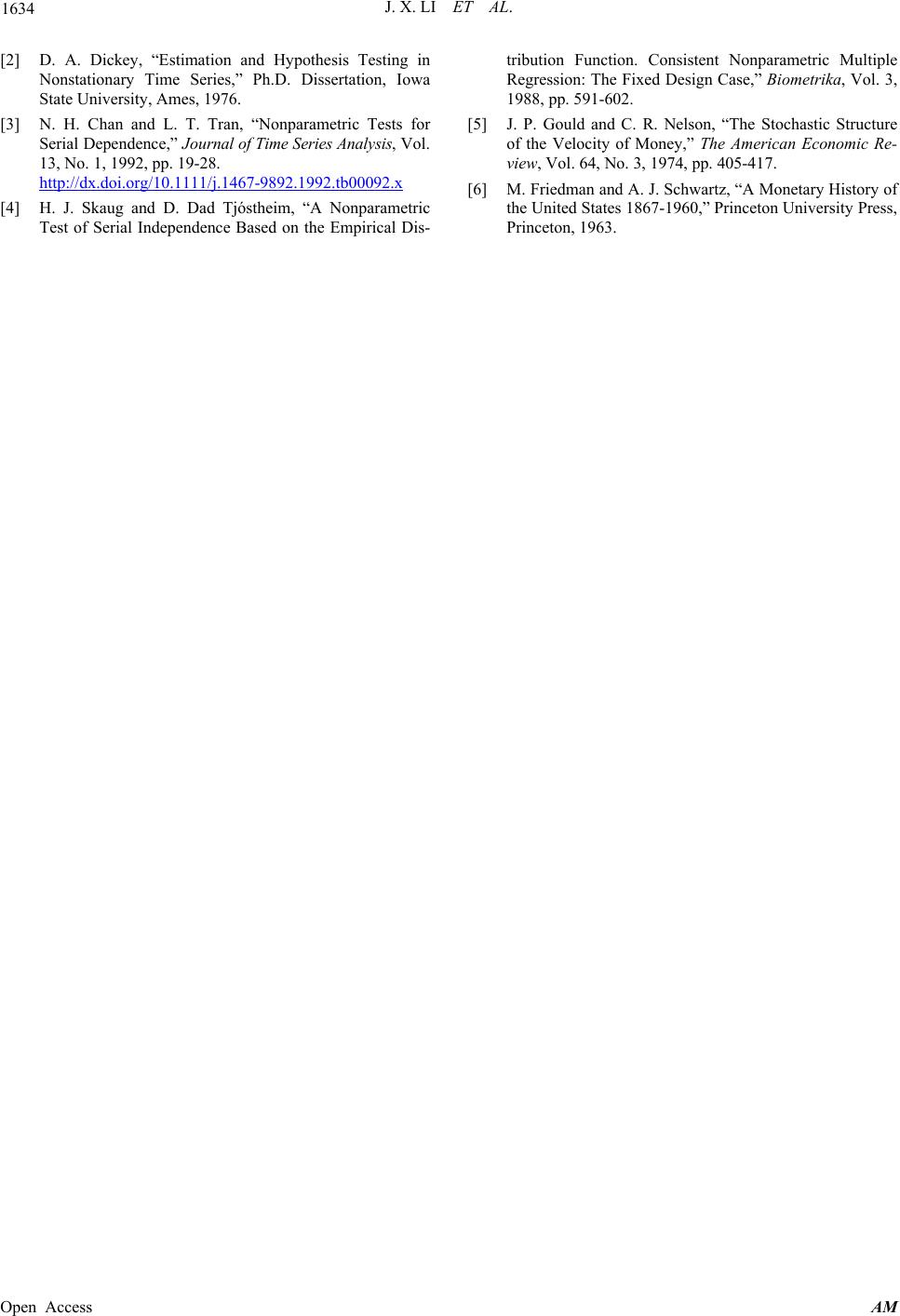 J. X. LI ET AL. Open Access AM 1634 [2] D. A. Dickey, “Estimation and Hypothesis Testing in Nonstationary Time Series,” Ph.D. Dissertation, Iowa State University, Ames, 1976. [3] N. H. Chan and L. T. Tran, “Nonparametric Tests for Serial Dependence,” Jou rnal of Time Series Analysis, Vol. 13, No. 1, 1992, pp. 19-28. http://dx.doi.org/10.1111/j.1467-9892.1992.tb00092.x [4] H. J. Skaug and D. Dad Tjóstheim, “A Nonparametric Test of Serial Independence Based on the Empirical Dis- tribution Function. Consistent Nonparametric Multiple Regression: The Fixed Design Case,” Biometrika, Vol. 3, 1988, pp. 591-602. [5] J. P. Gould and C. R. Nelson, “The Stochastic Structure of the Velocity of Money,” The American Economic Re- view, Vol. 64, No. 3, 1974, pp. 405-417. [6] M. Friedman and A. J. Schwartz, “A Monetary History of the United States 1867-1960,” Princeton University Press, Princeton, 1963.
|