Journal of Computer and Communications, 2013, 1, 14-18
Published Online December 2013 (http://www.scirp.org/journal/jcc)
http://dx.doi.org/10.4236/jcc.2013.17004
Open Access JCC
Comparison of Calibration Curve Method and Partial
Least Square Method in the Laser Induced Breakdown
Spectroscopy Quantitative Analysis
Zhi-bo Cong, Lan-xiang Sun*, Yong Xin, Yang Li, Li-feng Qi
Lab. of Networked Control Systems, Shenyang Institute of Automation, Chinese Academy of Sciences, Shenyang 110016, China.
Received August 2013
ABSTRACT
The Laser Induced Breakdown Spectroscopy (LIBS) is a fast, non-contact, no sample preparation analytic technology; it
is very suitable for on-line analysis of alloy composition. In the cop per smelting ind ustry, analysis and control of the
copper alloy concentration affect the quality of the products greatly, so LIBS is an efficient qua ntitative analysis tech-
nology in the copper smelting industry. But for the lead brass, the components of Pb, Al and Ni elements are very low
and the atomic emission lines are easily submerged under copper complex characteristic spectral lines because of the
matrix effects. So it is difficult to get the online quantitative result of these important elements. In this paper, both the
partial least squares (PLS) method and the calibration curve (CC) method are used to quantitatively analyze the laser
induced breakdown spectroscopy data which is obtained from the standard lead brass alloy samples. Both the major and
trace elements were quantitatively analyzed. By comparing the two results of the different calibration method, some
useful results were obtained: both for major and trace elements, the PLS method was better than the CC method in
quantitative analysis. And the regression coefficient of PLS method is compared with the original spectral data with
background interference to explain the advantage of the PLS method in the LIBS quantitative analysis. Results proved
that the PLS method used in laser induced breakdown spectroscopy was suitable for simultaneous quantitative analysis
of different content elements in copper smelting indu s try.
Keywords: Laser-Induced Breakdown Spectroscopy (LIBS); Partial Least Square Method (PLS); Matrix Effects;
Quantitative Analysis
1. Introduction
In the field of metallurgical industry, current and the con-
ventional analysis methods are chemical analysis, spark
atomic emission spectrometry, flame a tomic absorption
spectrometry and so on. These methods require the sam-
ple pretreatment and analysis process is more complex,
thus increasing the metallurgical production time and
causing a great deal of energy and material waste. Laser
Induced Br e akd own Spectroscopy (LIBS) is an emission
spectrum analysis technology which uses a pulse laser as
the energy source and both qualitative and quantitative
analysis of elements can be achieved [1,2]. It is a fast,
noncontact, no sample preparation analysis technology
and becomes a hot topic in the field of spectral analysis
in recent years [3-5]. In th e copper smelting industry, the
lead brass has excellent cutting performance, wear resis-
tance and high strength, and it is widely used in valve,
lock, clock and watch manufacturing industry. But th e
lead brass is a complex copper alloy composed of a va-
riety of elements. It has two main content elements Cu
and Zn. Meanwh ile the Ni, Al, Pb, Sn elements have a
decisive role to its heat resistance, corrosi on resistance,
strength and ductility. The concentrations of main con-
tent elements and other elements differed by several or-
ders of magnitude cause a great matrix effects. So as the
conventional LIBS quantitative analysis method, the Ca-
libration Curve (CC) method has the poor accuracy.
Partial least squares (PLS) is a set of multivariate li-
near regressio n (MLR) and principal component regres-
sion (PCR) basic func tions method. It is a pattern recog-
nition method that has powerful processing ability of
high dimension data. It has been widely used in the bio-
medical, pharmaceutical, social science and other fields
[6-8]. In this paper, the PLS method was used to over-
come the multiple correlatio ns between variables of the
spectroscopic data and lead brass LIBS complex spectra
*
Corresponding author.

Comparison of Calibration Curve Method and Partial Least Square Method
in the Laser Induced Breakdown Spectroscopy Quantitative Analysis
Open Access JCC
15
were quantitatively analyzed. PLS method was compared
with the traditiona l calibration curve(CC) method to ve-
rify the superiority in the LIBS quantitative analysis.
2. Experiment
The experimental device set is shown in the Figure 1.
The ND: YAG laser made by BigSky Company is plas-
ma excitation source, the output wavelength is 1064 nm,
the maximum output energy is 200 mJ. The pulse laser
produced plasma at the sample surface through a 75 mm
focal lens. Detection device is composed of 4 piece of
Ocean Optics company HR2000+ spectrometer, the opt-
ical resolution of 0.1 nm (FWHM), the integration time is
1ms, the measurement wavelength rang e is 199 - 631 nm.
The ti ming controller is made by us to control Q delay of
laser device and delay between spectrometer and laser
device, the Q delay range is 120 μs - 220 μs, adjustable
step is 5 μs, spectral acquisition delay range is 0 μs - 10
μs, adjustable step is 0.1 μs. The analyzed lead brass sam-
ple is spectral purity Chinese standard sample; the GB
number is GSB 04-2416-2008. The Composition is shown
on the “Ref. (Reference) line” in Table 1.
In this experiment, the laser pulse energy is 95 mJ,
pulse frequency is 10 Hz. The spectral acquisition delay
is 2.4 μs to eliminate the background noise caused by
bremsstrahlung in the early stage of plasma [9]. Each
sample was measured 10 times in 5 different locations
separately, in order to prevent the e rror caused by inho-
mogeneous in its internal composition. Before the data
collection, there are 10 excitation pulses for ablation the
surface of the sample to clean the oxide impurities. There
is not any pretreatment process in the whole experiment.
The LIBS data of 6 samples is 300. Each sample data is
50, 40 of them used to establish the quantitative calibra-
tion model, the other 10 data for prediction to validate
the performance of quantitative methods.
3. Result and Discussion
3.1. Calibration Curve (CC) Method
The experimental spectral data is shown in Figure 2.
Most characteristic spectral lines are in the range 200 -
300 nm. Access to the National Institute of Standards and
Technology (NIST) atomic emission spectrum database,
the higher intensity and can be resolved element spectral
peaks is : Cu 324.754 n m, Pb 280.1995 nm, Al 257.5094
nm, Ni 221.6482 nm. These characteristic spectral lines
are used for calibration curve (CC) method quantitative
analysis.
Figure 1. Schematic diagram of the LIBS experimental set-
up.
Table 1. Predicted VS. Reference concentration (wt%) of all elements By PLS and CC method.
No. Cu Pb Ni Al
1
Ref. 59.98 0.414 1.474 0.075
PLS Pre.(M ± SD) 60.09 ± 0.22 0.418 ± 0.085 1.449 ± 0.065 0.076 ± 0.069
CC Cal.(M ± SD) 59.72 ± 1.03 0.11 ± 0.089 1.141 ± 0.158 0.198 ± 0.023
2
Ref. 57.77 0.76 0.795 0.0116
PLS Pre.(M ± SD) 58.03 ± 0.22 0.874 ± 0.088 0.849 ± 0.067 0.081 ± 0.071
CC Cal.(M ± SD) 59.39 ± 1.49 0.472 ± 0.138 0.353 ± 0.253 0.02 ± 0.003
3
Ref. 57.09 1.421 0.347 0.177
PLS Pre.(M ± SD) 57.25 ± 0.22 1.442 ± 0.088 0.369 ± 0.067 0.236 ± 0.0715
CC Cal.(M ± SD) 56.73 ± 0.84 1.222 ± 0.234 0.137 ± 0.125 0.013 ± 0.0814
4
Ref. 58.64 1.81 0.104 0.452
PLS Pre.(M ± SD) 59.02 ± 0.23 1.869 ± 0.092 0.196 ± 0.07 0.519 ± 0.075
CC Cal.(M ± SD) 61.27 ± 2.12 1.498 ± 0.261 0.021 ± 0.072 0.956 ± 0.183
5
Ref. 58.76 2.405 0.0286 0.761
PLS Pre.(M ± SD) 58.56 ± 0.20 2.292 ± 0.081 0.073 ± 0.062 0.706 ± 0.065
CC Cal.(M ± SD) 59.49 ± 1.38 2.914 ± 0.268 0.32 ± 0.049 1.463 ± 0.142
6
Ref. 59.6 1.393 0.386 0.262
PLS Pre.(M ± SD) 59.60 ± 0.23 1.476 ± 0.089 0.479 ± 0.068 0.375 ± 0.0731
CC Cal.(M ± SD) 58.79 ± 1.46 1.967 ± 0.318 0.189 ± 0.092 0.151 ± 0.101

Comparison of Calibration Curve Method and Partial Least Square Method
in the Laser Induced Breakdown Spectroscopy Quantitative Analysis
Open Access JCC
16
Figure 2. The LIBS spectrum of lead brass.
The calibration curve of element Pb on the char acter is-
tic spectral line 280.2 nm is shown in Figure 3. The star
symbols in the figure represent the relationship between
concentration and average intensity of characteristic spec-
tral line. The vertical lines between the circle symbols
represent the standard deviation of the calibration data.
Calibration model is linear fitting and the correlation
coefficient “R” is 0.9776. The remaining 60 spectral data
are measured by this model.
Similarly, the other elements calibration curves and
measured data can be obtained by the same way. The
concentration measured of elements Cu, Pb, Ni and Al is
shown on the “CC Cal. (M ± SD) line” in Table 1. The
correlation coefficient R of calibration curve for Cu
(280.1995 nm) is 0.9176, for Ni(221.6482 nm) is 0.9687,
and for Al(257 .5 094 nm) is 0.9446. The conc entration
result shows that calibration curves method for lead brass
quantitative analysis is not good. That is because the
concentration of lead bras s are complex, the main ele-
ment Cu content is only about 60%, there are severe ma-
trix effects in the other elements measurement. Mean-
while the lead brass texture is very soft, which means the
laser ablation quality is different from each other every
time. So the result stability is also not good.
3.2. Partial Least Squares (PLS) Method
Using the same experimental data, quantitative analysis
was performed by partial least squares method. The in-
dependent variable is the LIBS spectral data obtained from
the exp eriment, from 199 to 631 nm there are totally
7895 spectral data points, namely there are 7895 dimen-
sions, the modeling data number is 240. The dependent
variable is the concentration of 4 elements, so there are 4
dimensions. The dependent variable is a multidimensional
matrix, so the model we used is PLS2 model. The full
cross-validation method is used to validate the model.
The detailed regression and verification method can be
reference literature about multivariate data analysis [10,
11].
In the PLS method, Selection of the number of Prin-
cipal Components (PC) depends on the residual Y va-
riance value in calibration model. The residual variance
shows the discrete degree of residual. With the increase
number of Principal Components, the Y residuals discrete
degree becomes lower. But much more numbers of PC
make the model more complex, and more systematic
noise will be introduced. So when the number of PC in-
creases, while the residual Y variance does not decrease
obviously, the number of PC is the most suitable for the
model. Figure 4 shows the relationship between Resi-
dual Y-variance and PCs of experimental data. When the
number of PC is 7, the residual Y variance is 0.0317, this
value is very small and residual Y variance does not de-
crease significantly as it increases. So the number of PC
of the PLS2 model is 7.
The relationship between predicted concentration and
reference concentration of element Pb by PLS2 model is
shown in the Figure 5. The correlation coefficient “R” is
0.9902, Root Mean Square Error of Prediction (RMSEP)
is 0.0911. In this model, the correlation coefficient “R”
between predicted concentration and reference concen-
tration of Cu is 0.9667, Ni is 0.9885, Al is 0.9554. The
result of predicted concentration is shown on the “PLS
Pre. (M ± SD) line” in Table 1. The PLS me thod results
and correlation coefficients showed very well.
Figure 3. Calibration curve of element Pb on line 280.2 nm.
Figure 4. Residual Y -variance VS. PCs.

Comparison of Calibration Curve Method and Partial Least Square Method
in the Laser Induced Breakdown Spectroscopy Quantitative Analysis
Open Access JCC
17
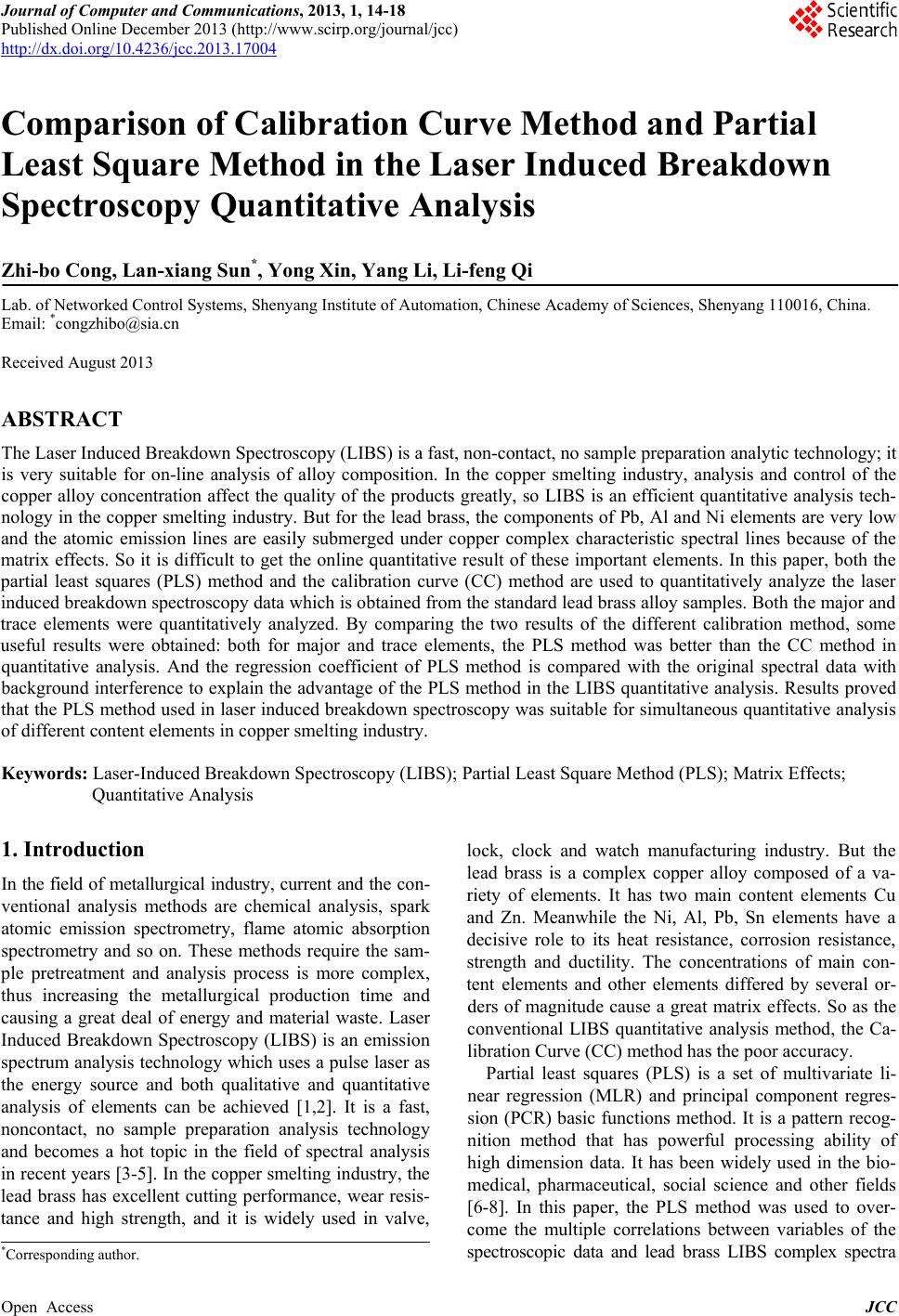
Figure 5. Predicted VS. Reference concentration (wt%) of
Pb.
3.3. The Advantage of PLS Method
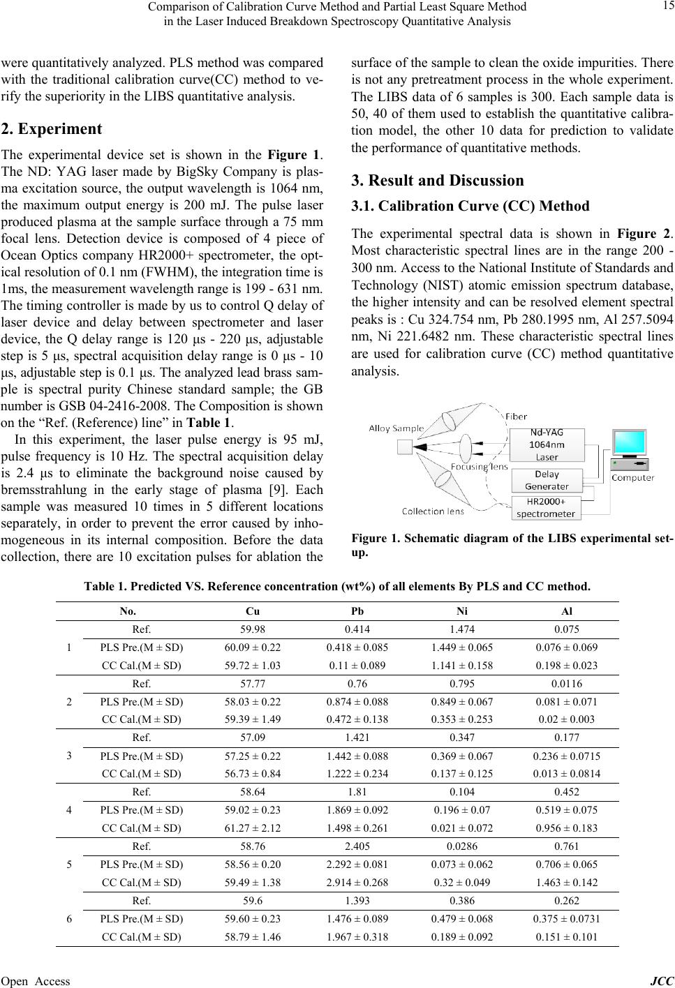
In PLS method, the regression coefficient means the re-
lationship between all independent variable X a nd de-
pendent variable Y, it can be calculated in the corres-
ponding number of principal components. In Section 3.2,
independent variable X (LIBS spectra data) and depen-
dent variable Y (element concentration) are used to es-
tablish the PLS calibration model. The regression coeffi-
cient between spectra data and element concen tration of
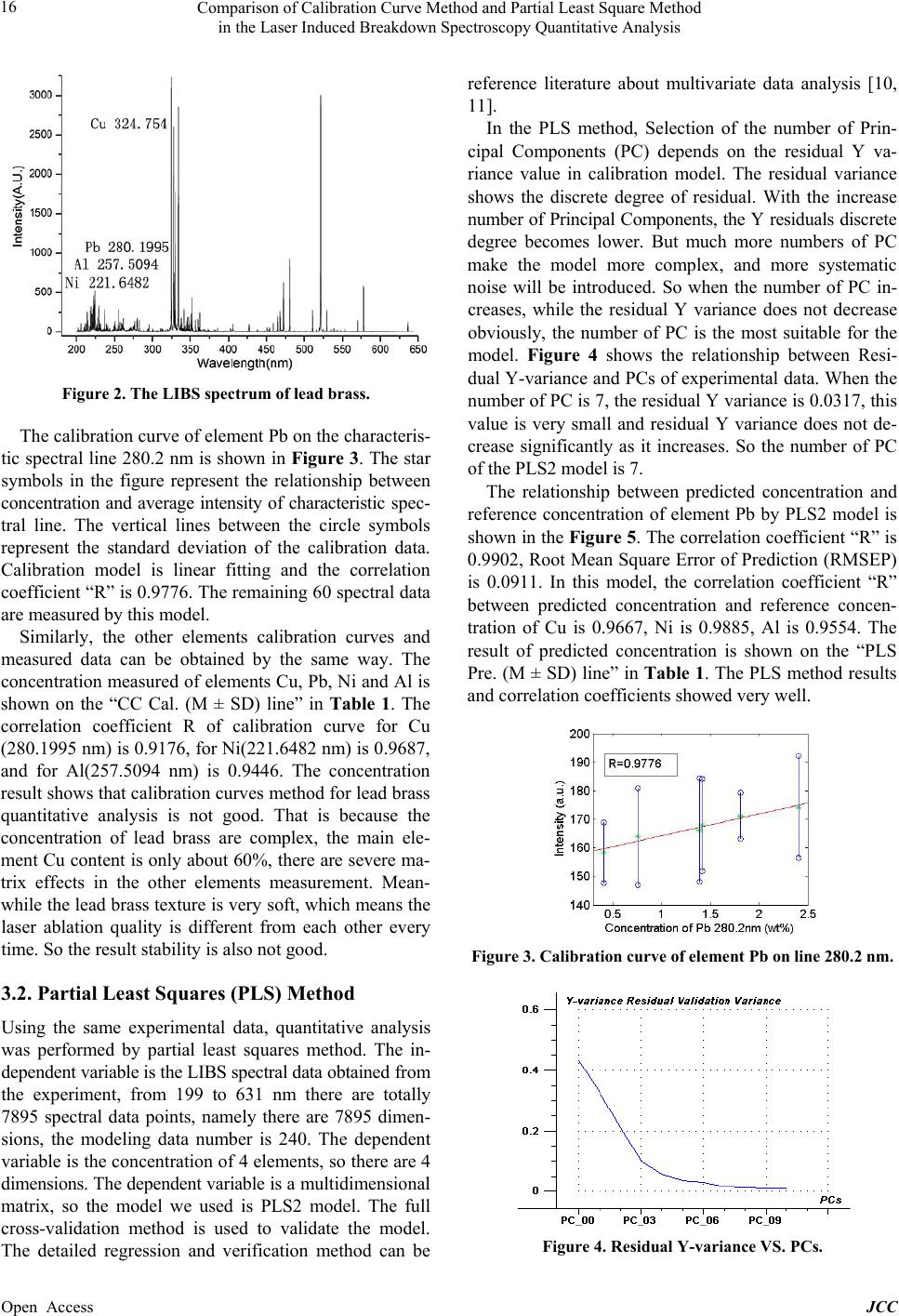
Al is shown in the Figure 6. The da rk line of Figure 6
means the regression coefficient with ordinate on the
right side, the light line means the spectra intensity with
ordinate on the left side. The spectral wavelength range
is 350 - 400 nm in the Figure 6. It can be observed that
at wavelength 394.25 nm and 396.06 nm, the regress ion
coefficient is 1.82 × 10−4 and 2.99 × 10−4, that is a larger
value. It means at this wavelength, the element concen-
tration and the spectra data have great correlation in PLS
model. Access to NIST, line 394.4 nm and 396.15 nm is
the Al characteristic spectral line. So in PLS model, in-
dependent variables and dependent variables have great
correlation at element characteristic spectral line (small
differences between the above wavelengths are caused by
error of spectrometer). But the intensity of spectra at the
same wavelength is weak and unstable. So the CC me-
thod calibration model using single spectral line intensity
is not good enough .
At wavelength 352.29 nm there is a peak but not Al
characteristic spectral line, it does not work in the CC
method Al calibration model. The regression coefficient
at the same wavelength is −0.92 × 10−4, it means the
spectral intensity and Al concentration are negative cor-
relation at this wavelength in PLS method calibration
model.
Unlike CC method to select the individual characteris-
tic peak, PLS method is to establish the relationship be-
Figure 6. The regression coefficient and spectrum of Al.
tween the intensity of full spectrum and element concen-
tration. By changing the independent variable space to
build a new principal components coordinate syste m, PLS
method establish positive or negative correlation rela-
tionship between all the spectral line intensity and ele-
ment concentrations. Then by selecting the number of
principal components to reduce the dimension of raw
data, PLS method establish a more stable quantitative
calibration model. We believe that this is the reason why
PLS quantitative calibration model is more effective than
CC method.
4. Conclusion
In this paper, both partial least squares and the calibra-
tion curve method were used to make the quantitative
analysis of LIBS spectral data of lead brass. After estab-
lishing the PLS calibration model, we can quickly get the
results of all the elements concentration. Compared with
the CC method, PLS method is more suitable for the
complicated matrix, element content different alloy.
5. Acknowledgements
This work has been sup po rted by the Equipment Devel-
opment Programs of the Chinese Academy of Sciences
(Grant No. YZ201247), the National High-Tech Research
and Development Program of China (863 Program) (Grant
No. 2012AA04060 8) and the National Natural Science
Fund (Grant No. 61004131).
REFERENCES
[1] J. P. Singh and S. N. Thakur, “Laser-Induced Breakdown
Spectroscopy,” Elsevier Science B.V., 2007.
[2] A. W. Miziolek, V. Palleschi and I. Schechter, “Laser-
Induced Breakdown Spectroscopy (LIBS): Fundamentals
and Applications,” Cambridge University Press, 2006.
http://dx.doi.org/10.1017/CBO9780511541261
[3] L. Zimmer, K. Okai and Y. Kurosawa, “Combined Laser
Induced Ignition and Plasma Spectroscopy: Fundamentals
and Application to a Hydrogen-Air Combustor,” Spec-

Comparison of Calibration Curve Method and Partial Least Square Method
in the Laser Induced Breakdown Spectroscopy Quantitative Analysis
Open Access JCC
18
trochim Acta, Part B, Vol. 62, 2007, pp. 1484-1495.
http://dx.doi.org/10.1016/j.sab.2007.10.024
[4] D. W. Hahn and N. Omenetto, “Laser-Induced Break-
down Spectroscopy (LIBS), Part II: Review of Instrumen-
tal and Methodological Approaches to Material Analysis
and Applications to Different Fields,” Appl. Spectrosc.,
Vol. 66, 2012, pp. 347-419.
http://dx.doi.org/10.1366/11-06574
[5] F. Sorrentino, G. Carelli, F. Francesconi, M. Francesconi,
P. Marsili, G. Cristoforetti, S. Legnaiol i, V. Palleschi and
E. Tognoni, “Fast Analysis of Complex Metallic Alloys
by Double-Pulse Time-Integrated Laser-Induced Break-
down Spectroscopy,” Spectrochim. Acta Part B, Vol. 64,
2009, pp. 1068-1072.
http://dx.doi.org/10.1016/j.sab.2009.07.037
[6] V. Lengard and M. Kermit, “3-Way and 3-Block PLS
Regressions in Consumer Preference Analysis,” Food
Quality and Preference, Vol. 17, No. 3-4, 2006, pp. 234-
242. http://dx.doi.org/10.1016/j.foodqual.2005.05.005
[7] A. Krishnan, L. J. Williams, A. R. McIntosh and H. Abdi,
“Partial Least Squares (PLS) Methods for Neuroimaging:
A Tutorial and Review”, NeuroImage, Vol. 56, No. 2,
2011, pp. 455-475.
http://dx.doi.org/10.1016/j.neuroimage.2010.07.034
[8] Y.-H. Chiang, “Using a Combined AHP and PLS Path
Modelling on Blog Site Evaluation in Taiwan,” Comput-
ers in Human Behavior, Vol. 29, No. 4, 2013, pp. 1325-
1333. http://dx.doi.org/10.1016/j.chb.2013.01.025
[9] Z. B. Cong, L. X. Sun, Y. Xin, H. Y. Kong and Z. J.
Yang, “Determination of Iron, Copper and Si licon in Al-
uminum Alloys by Laser Induced Break Down Spectros-
copy,” Vol. 31, No. 4, 2011, pp. 9-13.
[10] S. Wold, M. Sjöström and L. Eriksson, “PLS-Regression:
A Basic Tool of Chemometrics,” Chemometrics and In-
telligent Laboratory Sy stems, Vol. 58, No. 2, 2001, pp.
109-130. http://dx.doi.org/10.1016/S0169-7439(01)00155
-1
[11] J. A. Lopes and J. C. Menezes, “Industrial Fermentation
End-Product Modelling with Multilinear PLS,” Chemo-
metrics and Intelligent Laboratory Systems, Vol. 68, No.
1-2, 2003, pp. 75-81.
http://dx.doi.org/10.1016/S0169-7439(03)00089-3