Journal of Computer and Communications, 2013, 1, 41-45
Published Online November 2013 (http://www.scirp.org/journal/jcc)
http://dx.doi.org/10.4236/jcc.2013.16008
Open Access JCC
41
Efficiency Analysis of the Autofocusing Algorithm Based
on Orthogonal Transforms
Przemysław Śliwiński, Krzysztof Berezowski, Piotr Patronik, Paweł Wachel
Institute of Computer Engineering, Control and Robotics, Wrocław University of Technology, Wrocław, Poland.
Received September 2013
ABSTRACT
Efficiency of the autofocusing algorithm implementations based on various orthogonal transforms is examined. The
algorithm uses the variance of an image acquired by a sensor as a focus function. To compute the estimate of the vari-
ance we exploit the equivalence between that estimate and the image orthogonal expansion. Energy consumption of
three implementations exploiting either of the following fast orthogonal transforms: the discrete cosine, the Walsh-Ha-
damard, and the Haar wavelet one, is evaluated and compared. Furthermore, it is conjectured that the computation pre-
cision can considerably be reduced if the image is heavily corrupted by the noise, and a simple problem of optimal word
bit-length selection with respect to the signal variance is analyzed.
Keywords: Auto-Focusing; Image Variance; Disc re t e Orthogonal Transform s; Word-Length Selection; Architectural
Performance Evaluation
1. Introduction
We say that the image is sharp (in focus) when it is the
most detailed representation of the actual scene seen via
a lens. This intuitive observation led to many heuristic
algorithms which measure, like for instance (see e.g.
[1-3]):
• the variance of the image,
• the sum of squared Laplacian of the image, or
• the sum of squared values of the image transform by
selected edge-detection algorithms.
In this work we consider the first measure for the fol-
lowing rea sons:
• it can be shown that the variance of the image pro-
duced by the lens is a unimodal function which has a
maximum when the image is in focus. Moreover,
• the variance can effectively be estimated even in the
presence of a random noise.
Automatic focusing seems to not only be a desired fea-
ture of consumer electronic devices like digital cameras
and camcorders, but also an important tool used in secu-
rity or industrial app lications (like surveillance or micro-
scopy; cf. [1,4]). The focusing algorithm whose efficien-
cy we ex amine is a passive algorithm (that is, i t does not
require additional equipment) and operates on the data
acquired by the image sensor; see e.g. [5]. We use a va-
riance of the image data as the focus function and to find
its (single) maximum (i.e. to get the sharpest image) we
employ the golden section search (GSS) algorithm; see
[6]. Note that fast yet precise focusing in both surveil-
lance and microscopy is rather cumbersome since we
have to deal there with a thin depth-of-focus (DOF) issue
(in the former, it comes from application of large aper-
ture (fast) lenses while in the latter, this is a consequence
of short distances between a scene and a lens). A thin
DOF makes the maximum search problem much harder
since it typically implies a flat-tailed focus function with
a steeply-sloped peek whose unimodality is easily vi-
olated in a noisy environment.1
We begin with a problem statement and a focus func-
tion formula. Next, we present the focusing algorithm
and three implementations of the variance estimate com-
putatio n ro utines based on either:
• the discrete cosine,
• the Walsh-Hadamard, or
• the Haar wavelet orthogonal transforms, respectively.
Then, we experimentally establish the energy effi-
ciency of each implementation using an ARM processor
simulator. Finally, we shortly examine the minimum
word-length selection as a denoising algorithm in the
1In the shape from focus (SFF) applications, where the three dimen-
sional (3D) scene is reconstructed from a sequence of two-
dimensional
(2
D) images focused at the different distances, thinner DOFs enable
higher accuracy reconstructions; see e.g. [3,7,8].

Efficiency Analysis of the Autofocusing Algorithm Based on Orthogonal Transforms
Open Access JCC
42
presence of a thermal (Gaussian) noise.
2. Autofocusing Algorithm
The proposed algorithm can be considered as the solution
to a stochastic approximation problem. The captured
scene, the lens system and the image sensor are modelled
as follows; see Figure 1 and cf. [5]):
1) The scene is a 2D homogenous second-order sta-
tionary process with unknown distribution and unknown
correlation function ; cf. [ 9].
2) The lens has a circular aperture system that satisfies
the first-order optics laws, and is represented by a cen-
tered moving average filter of order proportional to the
distance
vs −
of the sensor from the image plane and
to the size of the lens aperture
D
; cf. [10].
3) The image sensor acts as an impulse sampler on the
lens-produced process.
The autofocusing algorithm simply seeks for the maxi-
mum of the focus function, which in our case is the va-
riance of the image produced by the lens for a given
scene. The assumptions above allow demonstrating the
unimodality property of this focus function, and hence,
enable an application of the simple golden-section search
algorithm to find the maximum. Since, for a given scene,
lens and a sensor, the number of steps performed by the
GSS algorithms is the same, it suffices to compare effec-
tiveness of the variance estimation implementations in
order to assess the effectiveness of the whole AF algo-
rithm.
We will now present the equivalence between the va-
riance estimate and the orthogonal expansion of the im-
age data. Thanks to this equivalence we can not only
compute the estimate (which can clearly be computed
directly from a standard variance estimate formula), but
we can also interpret the image as a regression function
(which can in turn be estimated separately in order to
remove the noise from the image). For simplicity we
examine the one-dimensional case (which can be justi-
fied by the symmetry argument since, by Assumption 2,
the lens aperture is circular).
Figure 1. A block diagram of the AF circuit [5].
Let
[ ]
T
N
xxX 
1
=
be the vector representing the raw
image (i.e. a sample function of the process produced by
the lens). The variance of such an image can be estimated
by the standard formula
.var
2
1
12
1
1





−=
∑∑
=
−
=
−n
N
n
n
N
nxNxNX
(1)
Also, the ve ctor
X
can be expanded in a discrete or-
thogonal series
{ }
k
ϕ
,
Nk ,,1 =
, so that
( )( ) ./ where,/
1
1
1
NnxNNkX
kn
N
n
kkk
N
k
ϕαϕα
∑∑
=
−
=
==
By the Parseval’s identity, we have that
.
2
2
2
1
2
1
1k
N
k
n
N
n
xN αα
∑∑ ==
−
+=
Hence, if the first term
1
ϕ
of the orthogonal series
expansion is a constant function (as it is the case in all
thre e cons idered series ), then we can easily ascertain that
the squared value of the first expansion coefficient
,
1
1
1n
N
n
xN∑
=
−
= α
equals to second term in the variance
estimate (1). As a result, we obtain the equivalent va-
riance estimation formula
,var
2
2k
N
k
X α
∑
=
=
in which the expansion coefficients
{ }
k
α
are computed
using the appropriate fast transform algorithm [11,12].
3. Orthogonal Transforms
Here we recollect some basic properties of the consi-
dered transforms. Each of them has the corresponding
matrix representation
,AXY=
where
A
is a square
NN×
orthogonal matrix (i.e. a
matrix of the unit spectra l nor m,
1
2=A
) and
[ ]
T
N
Y αα 
1
=
is the vector collecting the transformed
image (i.e. the transform coefficients).
3.1. DCT Transform Matrix
The matrix of the discrete cosine transform (DCT) con-
sists of the cosine basis functions sampled at the uniform
grid. The matrix is orthogonal and with entries; see e.g.
[12,13]:
[ ] .1,,0,,
2
1
cos, −=












+=Nnkn
N
k
nkA 
π
Observe that:
• The matrix dimension
N
is an arbitrary natural num-
ber (i.e. it is not restricted to powers of two like the
remaining transforms (this is because the orthogonal
systems of the trigonometric functions remain ortho-

Efficiency Analysis of the Autofocusing Algorithm Based on Orthogonal Transforms
Open Access JCC
43
gonal on a uniform dis c re te grid [14,15]).
• The matrix entries are real numbers, that is, in the
transform computations their trunc ated (approximated)
values are used.
• A direct implementation h as a polynomial complexity
( )
2
NO
.
• The Fast Discrete Cosine Transform is an in situ al-
gorithm and requires only
( ) NNO log
operations,
i.e., can be computed in a linearithmic (i.e. quasili-
near) time.
Example 1: For
4=N
the DCT matrix takes the
form
.
22222222
2222
22222222
2222
22
1














−−++−−
−−
+−−−−+
=A
3.2. Walsh-Hadamard Transform Matrix
The matrix of the Walsh-Hadamard (W-H) transform has
the following properties; see e.g. [11,16]:
• The matrix dimension
N
is a dyadic natural number
(i.e. it is a power of two).
• The entries are equal either
1
or
1−
, i.e. there is no
multiplication in the transform algorithm.
• A direct implementation h as a polynomial complexity
( )
2
NO
.
• The Fast Walsh Transform is an in situ algorithm and
requires
( ) NNO log
operations, i.e., can also be
computed in a linearithmic (i.e. quasilinear) time.
Example 2: For
4=N
the W-H matrix takes the form
.
1111
1111
1111
1111
2
1












−−
−−
−−
=A
3.3. Haar Transform Matrix
The matrix corresponding to the Haar Wavelet Trans-
form algorithm is somehow unique when compared to
the former two. In particular:
• A direct implementation results in a linearithmic
complexity
( ) NNOlog
.
• The Fast Haar Transform requires merely
( ) NO
operations, i.e., it can be computed in a linear time
(its lifting version can furthermore be computed in
situ). Neverthe l e ss ,
• Its dimension is an integral power of two (like in the
W-H case—in orde r t o p r e se rve ortho g ona lity).
• The entries are not integer like in the DCT case (they
are integral powers of
2
instead).
Example 3: The matrix of the four-point Haar trans-
form has the following entries; see e .g. [12]:
.
2200
0022
1111
1111
2
1












−
−
−−
=A
Note that the Haar transform matrices become sparser
(i.e. they have more-and-more zero entries) as their di-
mensions grow.
4. Energy Consumption Evaluation
From the formal point of view, all implementations are
equivalent, that is, given the same image data, they al-
ways yield the same value of the variance estimate.
However, different numerical properties of the trans-
forms suggest that the energy consumption of each im-
plementation may vary significan tly.
In order to verify this conjecture, we measured expe-
rimentally the energy consumptions of the variance cal-
culation. The experiments were run on two sample pic-
tures (Figure 2). The pictures were scaled to three sizes:
3232×
,
6464×
, and
128128×
, and converted to 8-bit
grayscale bitmaps. We used the DCT, Walsh-Hadamard
and Haar transforms implemented in the FXT library,
[17], and compiled them with the standard GCC compi-
ler.2 For our energy consumption assessment we em-
ployed the Panalyzer simulator of the ARM processor,
which is a popular SimpleScalar simulator augmented
with the power models of this processor.3
The calculations were performed using the double pre-
cision floating-po int numbers. Additionally, in attempt to
exploit the specifics of the Walsh-Hadamard transform,
we calculated the variance using the fixed-point imple-
mentation with the help of a separate integer number
routine4. In all simulations, we measured the total energ y
consum ption of the p roc essor m i c roa r c hi tecture.
The results are shown in Figure 3. Clearly, the energy
consumption does not depend on the particular image
and grows with the image size. Moreover:
• The implementation based on the Haar transform was
the most efficient energy consumption-wise.
• Next in order was the implementation based on the
DCT transform.
• The least efficient was the Walsh-Hadamard trans-
form-based implementation, both in floating- and
fixed-point versions.
While it seems to be obvious that the Haar transform
implementation has the best efficiency (as the result of
the transform’s linear computational complexity), the
smaller energy consumption of the DCT implementation
in relation to the Walsh one is somehow surprising and
2GCC 4.0.1 com piler, all optimization options disabled.
3Sim-panalyzer 2.0.3; see http://web.eecs.umich.edu/ ~panalyzer/
4See: http://math.ewha.ac.kr/~jylee/SciComp/sc-crandall/ walsh.c

Efficiency Analysis of the Autofocusing Algorithm Based on Orthogonal Transforms
Open Access JCC
44
Figure 2. The two sample images I and II.
Figure 3. Energy consumption of the three implementations
measured in mJ for the processor clocked at 500 MHz.
requires further study (it can be related with e.g. a better
low-level optimization of the DCT transform in the FXT
library). In turn, the almost identical results of the fixed-
and floating-point Walsh implementations suggest that
only a very small fraction of energy is consumed by the
arithmetic instructions in relation to the whole algorithm.
5. Word-Length Selection and Denoising
In this section we consider the word-length problem (i.e.
the required precision of the data representation) in the
presence of noise. The stochastic nature of the noise na-
ture creates random ‘fake’ local maxima in the focus
function estimate in which the GSS algorithm can easily
stuck (see however the analysis of the GSS algorithm in
[18], where the probability of such an event is shown to
vanish with the growing number of pixels). The simplest
way to attenuate the influence of the noise is to average
multiple p ictures taken at each focus distance. This solu -
tion however results in a slower and more power con-
suming focusing routine. In embedded systems, one
should therefore prefer more energy efficient, single-
image, approaches based on e.g. nonpar ametric regres-
sion estimation; see [19,20].
Inspired by the one of the most prominent estimation
techniques, the wavelet shrinking, we examine here the
simple algorithm reducing the noise and based on the
word-length selection problem solution; cf. e.g. [21]. We
assume here that the additive random noise
k
ε
is i.i.d.
and has the Gaussian distribution
( )
2
,0
ε
σ N
. Thus, each
pixel value can be described as
.
nnn
ux ε +=
where
n
u
are the actual (noiseless) raw images. The un-
iformly quantized (i.e. finite precision) versions of
n
x
,
for
M
fractional bits, can be represented as
 
,
2
½2
Mnn
M
n
u
x++ =
ε
where
 
⋅
denotes the standard floor function.
To establish the minimum number of fractional bits
M
such that the inaccuracy in the final (transformed)
image imposed by the quantization error do not exceed
the variance error introduced by the noise
n
ε
, we con-
sider the following mean squared error (MSE) error of
the transformed image
( )
( )( ) ,
ˆ
2
ˆ
2
MSE
2
1
2
1
2
1
kk
N
k
kk
N
k
kk
N
k
EE
EY
αααα
αα
−+−≤
−=
∑∑
∑
==
=
where
{ }
k
α
are the pixels of the transformed image
computed from the noiseless raw image pixels
{ }
n
u
,
{ }
k
α
ˆ
are the pixels of the transformed image computed
in exact arithmetic from the noisy pixels
{ } ,
n
x
and
{ }
k
α
are its quantized versions. For simplicity we will
examine the above error for the Walsh-Hadamard trans-
form only. We have
[ ]
( ) [ ]
 
[ ] .,
2
½2 1
and ,,
1
ˆ
,,
1
1
1
1
nkA
u
N
nkAu
N
nkAu
N
Mnn
M
N
n
k
nn
N
n
k
n
N
n
k
++
=
+=
=
∑
∑
∑
=
=
=
ε
α
εα
α
Exploiting the orthonormality property of the trans-
form matrix
A
and the independence of the noise
n
ε
,
we obtain that
( )( )
( )
.2
ˆ
and
ˆ12
2
1
2
2
1
+−
==
≤−=− ∑∑ M
kk
N
k
kk
N
kNEE
αασαα
ε
Comparison of these two error terms yields the fol-
lowing w or d-l e ngth selection formula
,
2
loglog
2
2





−
=
ε
σ N
M
which guarantees that, given the number of fractional bits
is M, the quantization-induced inaccuracy does not ex-
ceed (in the MSE sense) the noise-induced inaccuracy.
Remark 1: Since the noise “occupies” the least signif-
icant bits which are truncated by the quantization, one
can expect that for the selected
M
the noise will also
be (partially) shrinked (this aspect needs however a more
careful further examination). Alternatively, one can also
consider performing the classic shrinkage algorithm on
the transformed image (prior to the variance calculation)
in order to remove the noise [19,20].

Efficiency Analysis of the Autofocusing Algorithm Based on Orthogonal Transforms
Open Access JCC
45
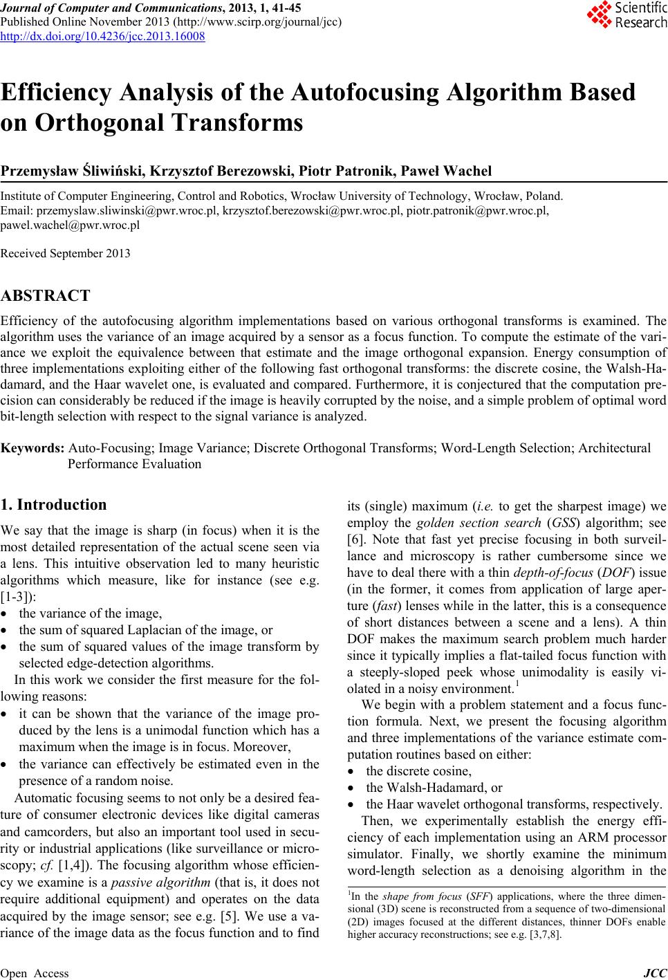
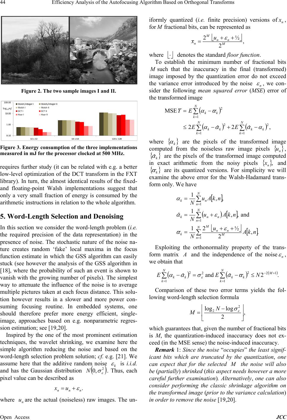
6. Final Remarks
In the paper we presented three implementations of the
image variance estimate evaluation which is the core and
the most computationally demanding part of the autofo-
cusing algorithm. We provided an experimental evidence
that the implementation based on the fast Haar transform
has a much better (by a wide margin) energy efficiency
than the remaining two implementations based on the
discrete cosine and the Walsh-Hadamard transforms.
Somehow unexpectedly, the experiments revealed that
there is no advantage of using the integer number Walsh-
Hadamard transform over the cosine one. Finally, having
in mind an ASIC implementation of the algorithm, we
also proposed the word-selection algorithm which deter-
mines the required precision of the image data with re-
spect to the size of the image data and to the variance of
the noise present in the data. The actual benefit of this
algorithm needs however to be verified experimentally.
Acknowledgements
The work is supported by the NCN gran t UMO-2011/01/
B/ST7/00666.
REFERENCES
[1] F. C. A. Groen, I. T. Young and G. Ligthart, “A Compar-
ison of Different Focus Functions for Use in Autofocus
Algorithms,” Cytometry, Vol . 6, No. 2, 1985, pp. 81-91.
http://dx.doi.org/10.1002/cyto.990060202
[2] M. Subbarao and J.-K. Tyan, “Selecting the Optimal Fo-
cus Measure for Autofocusing and Depth-from-Focus,”
IEEE Transactions on Pattern Analysis and Machine In-
telligence, Vol. 20, No. 8, 1998, pp. 864-870.
http://dx.doi.org/10.1109/34.709612
[3] A. N. R. R. Hariharan, “Shape-from-Focus by Tensor
Voting,” IEEE Transactions on Image Processing, Vol.
21, No. 7, 2012, pp. 3323-3328.
http://dx.doi.org/10.1109/TIP.2012.2190612
[4] E. Krotkov, “Focusing,” International Journal of Com-
puter Vision, Vol. 1, No. 3, 1987, pp. 223-237.
http://dx.doi.org/10.1007/BF00127822
[5] P. Śliwiński, “Autofocusing with the Help of Orthogonal
Series Transforms,” International Journal of Electronics
and Telecommunications, Vol. 56, No. 1, 2010, pp. 31-
37. http://dx.doi.org/10.2478/v10177-010-0004-5
[6] J. Kiefer, “Sequential Minimax Search for a Maximum,”
Proceedings of the American Mathematical Society, Vol.
4, No. 3, 1953, pp. 502-506.
http://dx.doi.org/10.1090/S0002-9939-1953-0055639-3
[7] S. K. Nayar and Y. Nakagawa, “Shape from Focus,”
IEEE Transactions on Pattern Analysis and Machine In-
telligence, Vol. 16, No. 8, 1994, pp. 824-831.
http://dx.doi.org/10.1109/34.308479
[8] K. S. Pradeep and A. N. Rajagopalan, “Improving Shape
from Focus Using Defocus Cue,” IEEE Transactions on
Image Processing, Vol. 16, No. 7, 2007, pp. 1920-1925.
http://dx.doi.org/10.1109/TIP.2007.899188
[9] J. W. Goodman, “Statistical Optics,” Willey-Interscience,
New York, 2000.
[10] S. J. Ray, “Applied Photographic Optics,” 3rd Edition,
Focal Pre ss , Oxford, 2004.
[11] K. Beauchamp, “Applications of Walsh and Related
Functions,” Academic Press, Waltham, 1984.
[12] W. H. Press, B. P. Flannery, S. A. Teukolsky and W. T.
Vetterling, “Numerical Recipes in C: The Art of Scientif-
ic Computing,” Cambridge University Press, Cambridge,
1993.
[13] D. Taubman and M. Marcellin, “JPEG2000. Image Com-
pression Fundamentals, Standards and Practice,” Kluwer
Academic Publishers, 2002, Vol. 642.
http://dx.doi.org/10.1007/978-1-4615-0799-4
[14] G. Szego, “Orthogonal Polynomials,” 3rd Edition, Amer-
ican Mathematical Society, Providence, RI, 1974.
[15] V. Mathews and G. Sicuranza, “Polynomial Signal
Processing,” Wiley, New York, 2000.
[16] B. Fino and V. Algazi, “Unified Matrix Treatment of the
fast Walsh-Hadamard Transform,” IEEE Transactions on
Computers, Vol. 100, No. 11, 1976, pp. 1142-1146.
http://dx.doi.org/10.1109/TC.1976.1674569
[17] J. Arndt, “Matters Computational: Ideas, Algorithms,
Source Code,” Springer-Verlag New York, Inc., New
York, NY, USA, 2010.
[18] P. Śliwiński and P. Wachel, “Application of Stochastic
Counterpart Optimization to Contrast-Detection Autofo-
cusing,” International Conference on Advances in Com-
puting, Communications and Informatics (ICACCI 2013),
Mysore, India, 22-25 August 2013, pp. 333-337.
http://dx.doi.org/10.1109/ICACCI.2013.6637193
[19] W. Härdle, G. Kerkyacharian, D. Picard and A. Tsybakov,
“Wavelets, Approximation, and Statistical Applications,”
Springer-Verlag, New York, 1998.
http://dx.doi.org/10.1007/978-1-4612-2222-4
[20] L. Györfi, M. Kohler, A. Krzyżak and H. Walk, “A Dis-
tribution-Free Theory of Nonparametric Regression,”
Springer-Verlag, New York, 2002.
http://dx.doi.org/10.1007/b97848
[21] G. Constantinides, P. Cheung and W. Luk, “Wordlength
Optimization for Linear Digital Signal Processing,” IEEE
Transactions on Computer-Aided Design of Integrated
Circuits and Systems, Vol. 22, No. 10, 2003, pp. 1432-
1442. http://dx.doi.org/10.1109/TCAD.2003.818119