Applied Mathematics
Vol.3 No.10A(2012), Article ID:24152,7 pages DOI:10.4236/am.2012.330216
Multigrid One-Shot Method for PDE-Constrained Optimization Problems
Group of Water Supply and Groundwater Protection, Institute IWAR, Department of Civil Engineering and Geodesy, Technical University of Darmstadt, Darmstadt, Germany
Email: s.hazra@iwar.tu-darmstadt.de
Received July 18, 2012; revised August 18, 2012; accepted August 25, 2012
Keywords: Shape Optimization; Simultaneous Pseudo-Time Stepping; Multigrid Methods; Preconditioner; Reduced SQP Methods; Reduced Hessian; One-Shot Method; Airfoil
ABSTRACT
This paper presents a numerical method for PDE-constrained optimization problems. These problems arise in many fields of science and engineering including those dealing with real applications. The physical problem is modeled by partial differential equations (PDEs) and involve optimization of some quantity. The PDEs are in most cases nonlinear and solved using numerical methods. Since such numerical solutions are being used routinely, the recent trend has been to develop numerical methods and algorithms so that the optimization problems can be solved numerically as well using the same PDE-solver. We present here one such numerical method which is based on simultaneous pseudo-time stepping. The efficiency of the method is increased with the help of a multigrid strategy. Application example is included for an aerodynamic shape optimization problem.
1. Introduction
Numerical methods for PDEs (also known as simulation techniques) are being used routinely for analysis of problems in scientific research and industrial applications as they are cost effective alternative to experiments. Since optimization of some quantity in such problems are quite common, recent trend in scientific research has been to develop numerical methods and algorithms so that the simulation techniques can be extended from analysis to simulation based optimization.The complexity and the nature of the optimization problem is completely different than those of the underlying PDEs. Therefore, it is not straight forward to extend the algorithms and solvers for PDE-solution to the PDE-constrained optimization problems. However, due to increasing interest in research in this field, continuous improvement is being reported by the researchers in this community.
The methods used for solving such optimization problems are mainly of two different types, namely, gradient based (such as steepest descent, quasi-Newton methods etc.) and gradient less (such as simulated annealing, genetic algorithm etc.). In general, gradient based methods are having advantage that they are much more efficient than the gradient-less methods. However, they only result in a local optimum. In comparison to that, gradient-less methods result in global optimum. Since in many applications a local minimum suffices for the purpose of solving the optimization problems, if it is achieved in considerable time, the gradient based methods are being considered there. The goal is to bring efficiency in the numerical methods for non-linear optimization so that the problems in real applications can be solved in “real time”.
When using a gradient based method, one has to compute the gradient by some means (such as using sensitivities or using adjoint equations etc.) [1]. Adjoint based gradient methods are advantageous as long as the number of design variables are large in comparison to the number of state constraints present in the problem. Solution of the adjoint equations can be obtained using almost the same computational effort as that of the forward or state equation. In “traditional” gradient methods (e.g., steepest descent or quasi-Newton methods), one has to solve the flow equations as well as the adjoint equations quite accurately in each optimization iteration. Despite using efficient CFD techniques, the over all cost of computation is quite high in these methods.
Due to this fact, in [2] we proposed a new method for solving such optimization problems using simultaneous pseudo-time stepping. In [3-6] we have applied the method for solving aerodynamic shape optimization problems without additional state constraints and in [7-9] applied the method to problems with additional state constraints. The overall cost of computation in all the applications has been between 2 - 8 times as that of the forward simulation runs, whereas in traditional gradient methods the cost of computation is between 30 - 60 forward simulation runs. This is a drastic reduction in computational cost. However, the number of optimization iterations is comparatively large since we update the design parameters after each time-step of the state and costate runs.
To overcome this problem, we use a multigrid strategy to accelerate the optimization convergence. The idea of the method is to solve optimization subproblems of similar structure at different grid levels. The solution of the coarse grid subproblem, which is cheap to compute, is used to find the optimal direction of the fine grid optimization problem efficiently. This method has been applied to aerodynamic shape optimization problems without additional state constraint in [10] and to problems with additional state constraint in [11]. The number of optimization iterations are reduced by more than 65% of that of single grid computations and the overall cost of computation of the optimization problem on fine grid is about 3 - 5 forward simulation runs. In this paper we present the whole idea in compact form, which otherwise can be found in detail in the references mentioned above and in [12].
The paper is organized as follows. In the next section we discuss the abstract formulation of the shape optimization problem and its reduction to the preconditioned pseudo-stationary system of PDEs. Section 3 presents the multigrid algorithm which we have used for the application example. Numerical result is presented in Section 4. We draw our conclusions in Section 5.
2. The Optimization Problem and Pseudo-Unsteady Formulation of the KKT Conditions
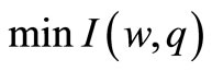
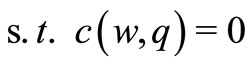
The optimization problems can be formulated mathematically in abstract form as (see, among others, in [1, 13-16], also in [2,3])
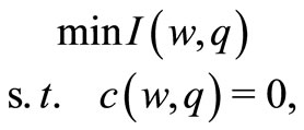 (1)
(1)
where 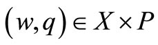 (X, P are appropriate Hilbert spaces), I: X × P → R and c: X × P → Y are twice Frechet-differentiable (with Y an appropriate Banach space).
The Jacobian, 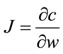 , is assumed to be invertible. Herethe equation c(w, q) = 0 represents the differential model equations, in our case the steady-state flow equations (Euler equations) together with boundary conditions, w is the vector of dependent variables and q is the vector of design variables. The objective I(w, q) for our application example is the drag of an airfoil.
The necessary optimality conditions can be formulated using the Lagrangian functional
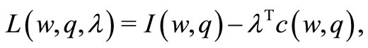 (2)
(2)
where λ is the Lagrange multiplier or the adjoint variable from the dual Hilbert space. If  is a minimum, then there exists a
  such that
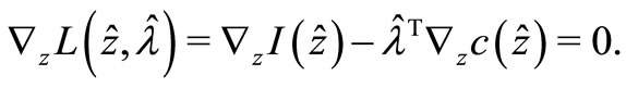 (3)
(3)
Hence, the necessary optimality conditions (known as KKT conditions) are
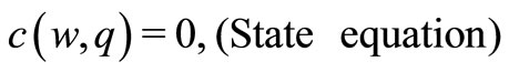 (4a)
(4a)
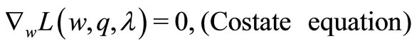 (4b)
(4b)
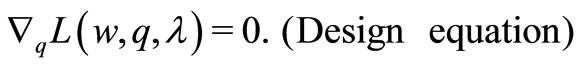 (4c)
(4c)
In adjoint based gradient methods the above system of equations are solved using some iterative techniques, for example, reduced SQP or rSQP methods. Instead of that, we use simultaneous pseudo-time stepping for solving above problem (4). In this method, to determine the solution of (4), we look for the steady state solutions of the following pseudo-time embedded evolution equations
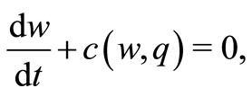
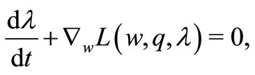 (5)
(5)
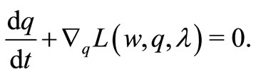
This formulation is advantageous, particularly for the problem class in which the steady-state forward (as well as adjoint) solution is obtained by integrating the pseudo-unsteady state equations (e.g. in our application example). However, pseudo-time embedded system (5) usually results, after semi-discretization, a stiff system of ODEs. Therefore explicit time-stepping schemes may converge very slowly or might even diverge. In order to accelerate convergence, this system needs some preconditioning. We use the inverse of the rSQP matrix (see, for example, [2] for details) as a preconditioner for the time-stepping process. Hence, the pseudo-time embedded system that we consider is
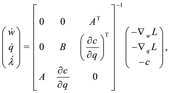 (6)
(6)
where A is the approximate Jacobian and B is the approximation of the reduced Hessian. Due to its block structure, the preconditioner is computationally inexpensive. As shown in [5], the reduced Hessian update based on most recent reduced gradient and parameter update informations is good enough for the problem class considered in the application example. We use the same update strategy here.
In many applications, the optimization problem contains additional state constraints. Treatment of additional state constraint in simultaneous pseudo-time stepping method is presented in detail in [7,9]. Adding a scalar state constraint to problem formulation (1) results in
 , (7)
, (7)
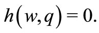
Typically, the additional constraint is of the form h(w, q) ≥ 0 however, for simplicity in the presentation we discuss only the equality constraint, which is also the case of our application example.
The preconditioned pseudo-time embedded non-stationary system to be solved in this case reads as
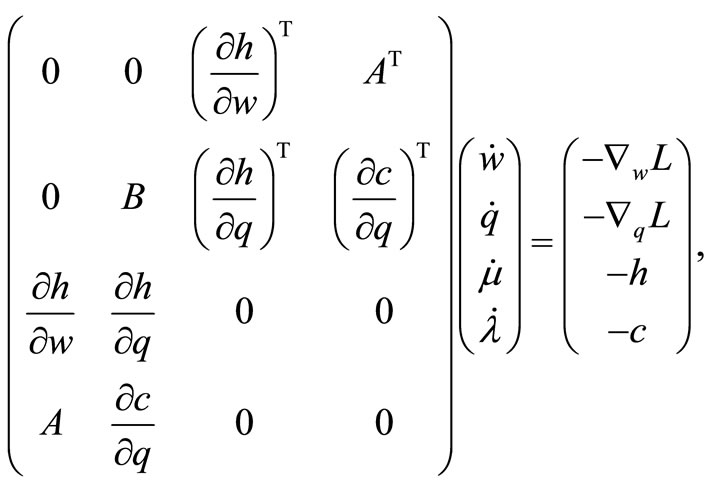 (8)
(8)
where μ is the Lagrange multiplier corresponding to the additional state constraint h(w, q).
Following the reduction strategy presented in [7,9], the solution of this problem is obtained in two steps. First, system (6) is solved for the design velocity . This design velocity is then projected onto the tangent space of the state constraint through the solution of the following QP
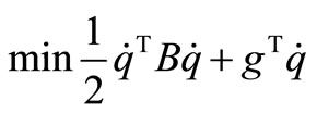
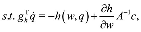 (9)
(9)
where 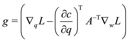
is the reduced gradient of the objective function and
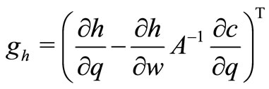
is the reduced gradient of the constraint h(w, q). For the construction of the reduced gradients g and gh, one has to solve one adjoint problem (approximately) for g and one for gh. Due to the nonlinearity of the problem, there is some deviation from the additional state constraint. Therefore we use a correction strategy in each optimization step to avoid this deviation. The correction strategy as well as the algorithm presented below can be found in [7,9].
The one-shot algorithm for solving this problem reads as follows:
Algorithm 1: The simultaneous pseudo-time stepping for the preconditioned system 0) Set ; start at some initial guess w0, λ0, μ0 and q0.
1) Compute λk + 1, μk + 1 marching one step in time for the adjoint equations.
2) Compute sensitivities using state and adjoint solutions.
3) Determine some approximation Bk of the projected Hessian of the Lagrangian.
4) Solve the quadratic subproblem (9) to get .
.
5) March in time one step for the design equation.
6) Use the correction step for the new qk + 1.
7) Compute wk + 1 marching one step in time for the state equations.
8) Set ; go to 1) until convergence.
3. The Multigrid Algorithm
As it is well-known, multigrid methods are iterative methods for solving system of algebraic equations, which results, for example, after discretization of PDEs. In these methods, iterative methods (such as Jacobi, GaussSeidel etc.) for linear system of equations having inherent smoothing properties are applied at different grid resolutions to remove the errors of all frequencies present in the system of equations leading to faster convergence of the method. Pioneering works, theories and applications of multigrid methods can be found, among others, in [17-21]. Similar ideas for the full optimization problems, also termed as “optimization-based” multigrid methods, are discussed in [22-25]. In our applications, we use similar strategy. The basic difference in our implementations is that we use multigrid in the context of simultaneous pseudo-time stepping. In the multigrid algorithm we solve different optimization subproblems on different grid levels. The coarse grid solution, which is achieved in much less computational effort, is used to accelerate the convergence of the optimization problem in fine grid. The solution methodology is based on simultaneous pseudo-time stepping as mentioned in the previous section. The ideas are demonstrated through practical aerodynamic shape optimization applications with Euler equations in 2D.
In the following algorithm, n denotes the current mesh resolution and N the next coarser mesh resolution;  denotes the prolongation operator and
  denotes the restriction operator. The multigrid algorithm reads as [11]
Algorithm 2:
1) If on the finest level, solve partially the optimization problem (7) and get  .
.
2) Compute  and
and  .
.
3) Compute  .
.
4) Solve in each coarse grid iteration the modified subproblem
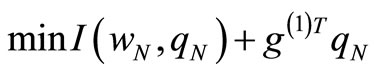
 (10)
(10)
to get the update vector
(as in steps 5) and 6) of Algorithm 1).
5) Compute 
6) Update  .
.
7) Goto step 3) in case of more than one coarse grid iterations.
Otherwise
8) Solve partially the problem (7) with initial solution  .
.
The algorithm defines the V-cycle template of the multigrid algorithm. The coarse grid subproblem contains objective function and the state constraints which are corrected using the in-exact reduced gradients. The steps based on coarse-grid subproblem leads to (faster) improvement of the optimal solution of the fine-grid problem maintaining the feasibility.
Multigrid computations start on the finest level. “Partially” solving means few iterations of the one-shot method. For prolongation we use linear interpolation and for restriction we use simple injection. Since problems (7) and (10) are of similar structure, all steps of Algorithm 1 can be carried out at respective discretization levels. Only for problem (10), step 6) of Algorithm 1 is carried out after the prolongation of the update vector to finest level. This has advantage that all the modules of the codes, developed in our earlier works, can be used in different discretization levels with minor modifications.
In the present paper, we have implemented this method for the shape design example using Euler equations. The details of governing equations, discretization, geometry parameterization, gradient computation and grid perturbation strategy can be found in [3,7].
4. Numerical Results and Discussions
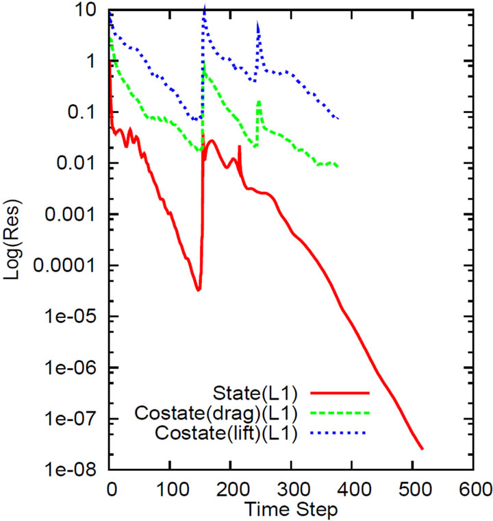
We present here the results of a test case of RAE 2822 airfoil for drag reduction with constant lift together with geometric constraint of constant thickness. The flow conditions are given at transonic Mach number 0.73 and angle of incidence 2 degrees. Further results obtained using this method can be found in [11]. The computational domain consists of C-grids in three levels with size: (321 × 57) (denoted by L1), (161 × 29) (denoted by L2) and (81 × 15) (denoted by L3). On these grid levels the preconditioned pseudo-stationary equations, resulting from the necessary optimality conditions corresponding to the optimization subproblems of Section 3, are solved using Algorithm 1. The initial values of the iterations (i.e., w0, λ0 and μ0) are obtained after 150 time steps on L1 level (and 100 time steps on L2 and L3 levels) of the state and costate equations. During a switch from “n” to “N” or from “N” to “n” the “restart” facility is used to read the solution of last iteration on the same level and this solution is corrected (as there is change in the geometry) using 85 time steps on L1 (and 55 time steps on L2 & L3) of the state and costate solvers (refer to figures of convergence histories). After the convergence of the optimization problem, another 200 time-steps are carried out (in L1) for the state equation to get more accurate values of the surface pressure and force coefficients.
The number of design parameters on three levels are 81 (L1), 41 (L2) and 21 (L3) respectively. In step (ii) of Algorithm 2, the reduced gradients are the sum of reduced gradients at levels L1 and L2. On the finest level, 5 iterations and on the next two coarser levels 6 and 2 iterations, respectively, are carried out. In the prolongation step from L3 to L2, 2 iterations are carried out. In the next restriction from L2 to L3, 2 iterations are carried out. In the next prolongation step from L3 to L2, 6 iteration as are carried out. The convergence of the optimization requires 2 W-cycles and in total 95 optimization iterations. For the same problem, computation on single grid (using Algorithm 1) requires 475 iterations (see in [11]). The drag reduction is about 62.16% and the lift is well maintained with a change of only 0.004%. These values are same as those of single grid computations. The optimization convergence history is presented in Figure 1, where the change in darg (top) and in lift (bottom) values during the optimization iterations appear. The convergence history of state and costate iterations are presented in Figure 2 at different grid levels. Comparison of cam ber lines, airfoils and surface pressure distributions are presented in Figure 3, where one can see in the surface pressure distributions (bottom) that the strong shock before optimization has been disappeared for the optimal profile. The number of optimization iterations depend on parameters chosen in the reduced Hessian updates. By fine tuning those parameters, same convergence criteria could
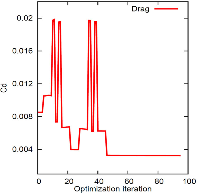
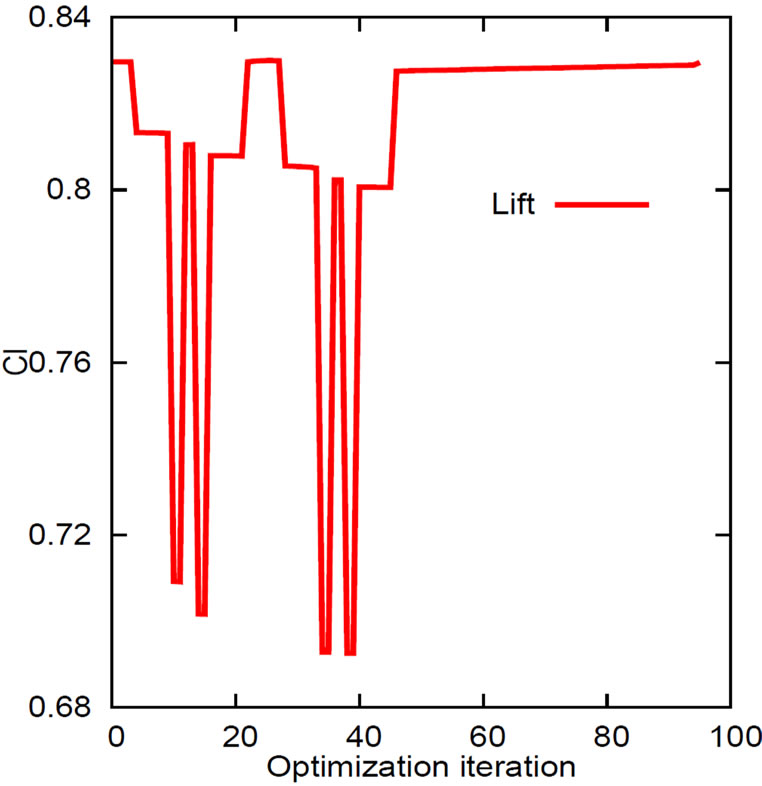
Figure 1. Convergence history of the optimization iterations.
 (a)
(a)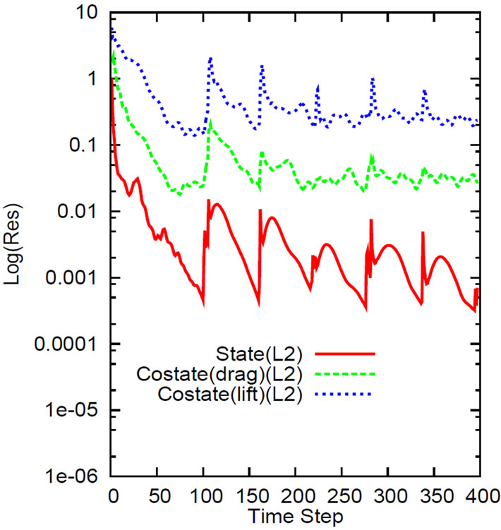 (b)
(b)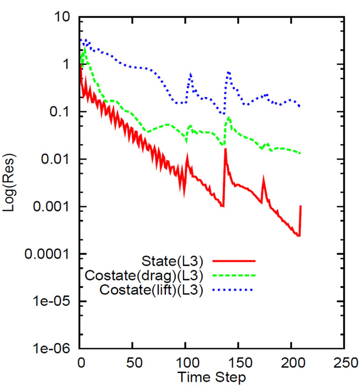 (c)
(c)
Figure 2. Convergence history of state and costate residuals on level-1 (a), level-2 (b) and level-3 (c).
be attained in 85 optimization iterations [11]. However, it is to note that the final converged solution remains the same. This is another proof of numerical stability of the method. Also in any case, the total effort is about 5 times that of the forward simulation runs, since one sufficiently converged forward solution needs about 450 time-steps and total effort in the finest level is less than four forward simulation runs. Adding up the time-steps required in coarser and coarsest level, we come up with this number.
5. Conclusion
One-shot multigrid strategy is explained and used for aerodynamic shape optimization. The preconditioned pseudo-stationary state, costate and design equations are integrated simultaneously in time at different discretiza-
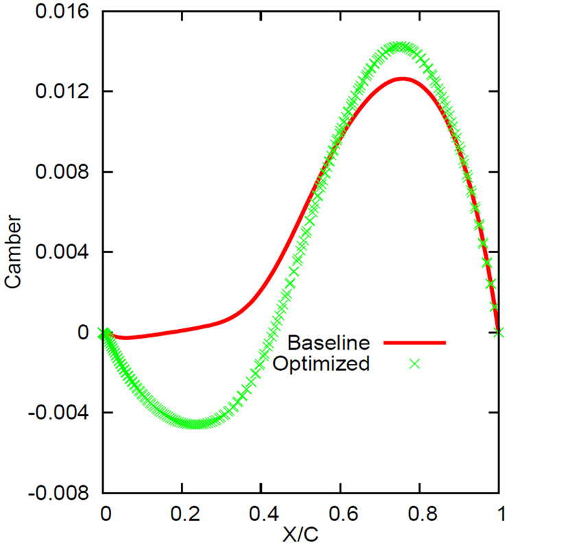
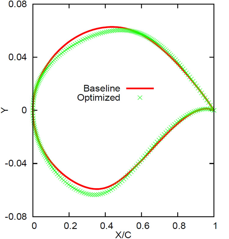
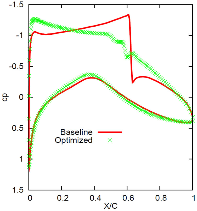
Figure 3. Comparison of Camberlines, airfoils and surface pressure distributions.
tion levels. Coarse grid solution, which is less expensive to compute, is used to accelerate the convergence of the optimization problem in fine grid. Multigrid strategy is quite effective when far away from the solution. The overall convergence is achieved by about 25% - 35% effort of that required by single grid computations using the same method.
6. Acknowledgements
I would like to thank DLR, Braunschweig, for giving access to the FLOWer code.
REFERENCES
- M. D. Gunzburger, “Perspectives in Flow Control and Optimization,” SIAM, Philadelphia, 2003.
- S. B. Hazra and V. Schulz, “Simultaneous Pseudo-Timestepping for PDE-Model Based Optimization Problems,” Bit Numerical Mathematics, Vol. 44, No. 3, 2004, pp. 457- 472. doi:10.1023/B:BITN.0000046815.96929.b8
- S. B. Hazra, V. Schulz, J. Brezillon and N. R. Gauger, “Aerodynamic Shape Optimization Using Simultaneous PseudoTimestepping,” Journal of Computational Physics, Vol. 204, No. 1, 2005, pp. 46-64. doi:10.1016/j.jcp.2004.10.007
- S. B. Hazra, “An Efficient Method for Aerodynamic Shape Optimization,” AIAA Paper 2004-4628, 10th AIAA/ISSMO Multidisciplinary Analysis and Optimization Conference, Albany, 2004.
- S. B. Hazra, “Reduced Hessian Updates in Simultaneous Pseudo-Timestepping for Aerodynamic Shape Optimization,” 2006.
- S. B. Hazra and N. Gauger, “Simultaneous PseudoTimestepping for Aerodynamic Shape Optimization,” Percent Allocation Management Module, Vol. 5, No. 1, 2005, pp. 743-744.
- S. B. Hazra and V. Schulz, “Simultaneous PseudoTimestepping for Aerodynamic Shape Optimization Problems with State Constraints,” SIAM Journal on Scientific Computing, Vol. 28, No. 3, 2006, pp. 1078-1099. doi:10.1137/05062442X
- S. B. Hazra, V. Schulz and J. Brezillon, “Simultaneous Pseudo-Timestepping for 3D Aerodynamic Shape Optimization,” Journal of Numerical Mathematics, Vol. 16, No. 2, 2008, pp. 139-161. doi:10.1515/JNUM.2008.007
- S. B. Hazra and V. Schulz, “Simultaneous PseudoTimestepping for State Constrained Optimization Problems in Aerodynamics,” in: L. Biegler, O. Ghattas, M. Heinkenschloss, D. Keyes and B. van Bloemen Waanders, Eds., Real-Time PDE-Constrained Optimization, SIAM, Philadelphia, 2007.
- S. B. Hazra, “Multigrid One-Shot Method for Aerodynamic Shape Optimization,” SIAM Journal on Scientific Computing, Vol. 30, No. 3, 2008, pp. 1527-1547. doi:10.1137/060656498
- S. B. Hazra, “Multigrid One-Shot Method for State Constrained Aerodynamic Shape Optimization,” SIAM Journal on Scientific Computing, Vol. 30, No. 6, 2008, pp. 3220- 3248. doi:10.1137/070691942
- S. B. Hazra, “Large-Scale PDE-Constrained Optimization in Applications,” Springer-Verlag, Heidelberg, 2010. doi:10.1007/978-3-642-01502-1
- J. L. Lions, “Optimal Control of Systems Governed by Partial Differential Equations,” Springer-Verlag, New York, 1971. doi:10.1007/978-3-642-65024-6
- O. Pironneau, “Optimal Shape Design for Elliptic Systems,” Springer-Verlag, New York, 1982.
- P. Neittaanmiaki, J. Sprekels and D. Tiba, “Optimization of Elliptic Systems,” Springer, Berlin, 2006.
- F. Troltzsch, “Optimal Control of Partial Differential Equations: Theory, Methods and Applications,” Graduate Studies in Mathematics, AMS, 2010.
- A. Brandt, “Multigrid Techniques: 1984 Guide with Applications to Fluid Dynamics,” SIAM, Philadelphia, 1984.
- W. Hackbusch, “Multigrid Methods and Applications,” Springer-Verlag, Berlin, 1985.
- P. Wesseling, “An Introduction to Multigrid Methods,” R. T. Edwards, Inc., Philadelphia, 2004.
- S. F. McCormick, “Multilevel Adaptive Methods for Partial Differential Equations,” SIAM, Philadelphia, 1989. doi:10.1137/1.9781611971026
- A. Jameson, “Solution of the Euler Equations for Two Dimensional Transonic Flow by a Multigrid Method,” Applied Mathematics and Computation, Vol. 13, No. 3-4, 1983, pp. 327-356. doi:10.1016/0096-3003(83)90019-X
- S. Ta’asan, “Multigrid One-Shot Methods and Design Strategy,” Lecture Notes on Optimization, 1997.
- S. G. Nash, “A Multigrid Approach to Discretized Optimization Problems,” Optimization Methods and Software, vol. 14, 2000, pp. 99-116. doi:10.1080/10556780008805795
- R. M. Lewis and S. G. Nash, “A Multigrid Approach to the Optimization of Systems Governed by Differential Equations,” 2000.
- R. M. Lewis and S. G. Nash, “Model Problems for the Multigrid Optimization of Systems Governed by Differential Equations,” SIAM Journal on Scientific Computing, vol. 26, no. 6, 2005, pp. 1811-1837. doi:10.1137/S1064827502407792