Technology and Investment
Vol.3 No.2(2012), Article ID:19391,13 pages DOI:10.4236/ti.2012.32011
Investment Timing with Incentive-Disincentive Contracts under Asymmetric Information*
1Graduate School of Social Sciences, Tokyo Metropolitan University, Tokyo, Japan
2Graduate School of Economics, Osaka University, Osaka, Japan
Email: tshibata@tmu.ac.jp, nishihara@econ.osaka-u.ac.jp
Received January 15, 2012; revised February 13, 2012; accepted February 21, 2012
Keywords: Real Options; Asymmetric Information; Incentive-Disincentive; Principal-Agent Problem
ABSTRACT
This paper examines a manager’s investment timing in the presence of asymmetric information between an owner and the manager. In particular, we extend the asymmetric information problem by incorporating not only an incentive but also disincentive. Investment timing is delayed more under asymmetric information than under symmetric information. However, investment timing under asymmetric information converges to the symmetric information investment timing by making the disincentive (penalty) for the manager’s untruthful report sufficiently large. Consequently, by adopting an enlarged set of incentive-disincentive contracts framework, we showed that there is a relationship between the symmetric and asymmetric information problems.
1. Introduction
In most modern corporations, owners delegate the corporate management to managers, taking advantage of managers’ special skills and expertise. In this situation, asymmetric information is likely to exist between them. Asymmetric information is a situation where a portion of the underlying state variable is privately observed by the managers, while it is unobservable by the owners. Managers with private information have an incentive to provide a false report and then divert free cash flow to themselves. Thus, asymmetric information leads to agency conflicts.
The real options model has become a standard framework for investment timing decisions in corporate finance. For the interested reader, Dixit and Pindyck [1] provide an excellent overview of the standard real options approach. The main result is to obtain the optimal investment timing and project value under uncertainty. In the standard real options model, however, there are no agency conflicts between owners and managers, because the firm is assumed to be managed by owners.1
Several studies have begun the task of incorporating agency conflicts into the real options model. Grenadier and Wang [2] (hereafter GW) develop models of investment timing in the presence of agency conflicts arising from asymmetric information between owners and managers.2 In such a situation, owners must design a contract to provide mechanisms for managers to reveal private information truthfully. They assume that the owners give the managers an incentive to reveal the managers’ private information. The implied investment timing is then delayed, compared with that under symmetric information, which leads to a decrease in the stock price (owners’ value). Although these strategies turn out to be suboptimal, they reduce the owners’ losses arising from asymmetric information. Without any mechanism that induces managers to reveal private information truthfully, owners suffer further distortions.
To the best of our knowledge, there has been little examination of such contracts other than the incentive mechanism in a real options model under asymmetric information. Owners may increase their own value by designing other mechanisms to induce managers to reveal private information truthfully. One important way is to use a disincentive mechanism. For example, because an owner audits a manager at a cost, the owner imposes penalties on the manager if an untruthful report by the manager is detected.3 Thus, it is natural to design an optimal contract containing both incentive and disincentive mechanisms. In most modern corporations, the disincentive system is designed so that owners can inspect managers’ behaviour.
Shibata [12] (hereafter, S) extends the model of investment timing developed by GW to design a contract with an incentive-disincentive mechanism, in which the owners induce the managers to reveal private information by giving bonuses and imposing penalties when an untruthful report is detected by randomized auditing. Obviously, the incentive-disincentive scheme in the S model expands on that of the incentive-only scheme in the GW model. Thus, the investment timing distortions in the S model are smaller than those in the GW model. Nevertheless, penalties are decided by the owners endogenously, and they are restricted to be less than the maximum amount of the managers’ diverted cash flows for untruthful reporting. These two features of the model are unreasonable in practice as follows. First, the penalties are specified not by the owners, but by legislation. Second, the penalties are not always restricted to be less than the maximum amount of the managers’ diverted cash flows. Suppose that, for example, although the managers divert free cash flows of 30,000 USD to themselves using their information advantage, the managers’ untruthful actions are detected during auditing. Then, in the S model, the managers are fined a penalty of 30,000 USD, which equals the diverted cash flow. However, in practice, a court applying the legislation can impose a penalty (e.g., 50,000 USD) of more than the diverted cash flow of 30,000 USD. Thus, it is reasonable that penalties are imposed on owners exogenously and that the penalties are not always less than the diverted free cash flows when untruthful reporting is detected during auditing.
This paper extends the model of investment timing with incentive-disincentive contracts under asymmetric information between owners and managers by eliminating the assumption that the penalties are less than the diverted cash flows. By assuming that penalties are imposed on the owners exogenously, the penalties may be smaller or larger than the diverted cash flows. Then, the set of incentive-disincentive contracts could be enlarged, compared with those in the S model. This paper highlights how the enlarged set of incentive-disincentive contracts influence investment timing, the stock price (owners’ value), and social welfare. In the existing papers discussed above, there is a divergence in investment timing and these values between the symmetric and asymmetric information cases. By adopting an enlarged set of incentive-disincentive contracts framework, our paper makes the first attempt to bridge the gap between the symmetric and asymmetric information cases.
In our results, the implied investment triggers (timings) can be derived in three feasible regions, depending on the magnitude of the exogenous penalties. The three feasible regions are the incentive-only (bonus-incentive only) region, the incentive-disincentive combination (bonus-incentive and audit-penalty) region, and the disincentiveonly (audit-penalty only) region. The investment trigger in the incentive-only region is equivalent to the one in the GW model. The investment trigger in the combination region includes the one in the S model. Most importantly, the symmetric information investment trigger of McDonald and Siegel [13] (hereafter MS) can be approximated by making the penalty for the manager’s false report sufficiently large. Consequently, by adopting an enlarged set of incentive-disincentive contracts framework, we show that there is a relationship between the symmetric and asymmetric information problems.
We analyse inefficiencies in investment timing, stock price (owners’ values), and total social welfare (loss) arising from asymmetric information. An increase in the penalty for managers’ cheating makes the suboptimal investment timing under asymmetric information approach the same as the optimal timing under symmetric information, which increases the stock price (i.e., increases the efficiency of the owners’ welfare). In contrast, an increase in the penalty does not necessarily rise the total social welfare. Thus, we conclude that an owner’s rationality does not necessarily increase total social rationality. In other words, an increase in the penalty does not necessarily increase the efficiency of the total social welfare while it always increases the efficiency of the owners’ welfare.
The paper proceeds as follows. Section 2 describes the framework of our model. It is useful to consider the symmetric information problem as a benchmark before analysing the asymmetric information problem. Section 3 provides the solution to the asymmetric information problem. We then discuss the properties of the solution. Section 4 investigates the numerical implications. Section 5 concludes. Technical developments are contained in two appendices. Appendix A contains proofs of the results in the paper. Appendix B contains the solutions to the optimization problems of GW and S to compare our results with theirs.
2. Model
In this section, we formulate our model. Subsection 2.1 describes the model framework. Subsection 2.2 formulates the asymmetric information problem. Subsection 2.3, as a benchmark, provides the solution to the symmetric information problem.
2.1. Setup
The owner of a firm has the option to invest in a single project. We assume that the owner (principal) delegates the investment decision to a manager (agent). Throughout our analysis, we assume that the owner and the manager are risk neutral and aim to maximize their expected pay-offs.
If the investment option is exercised at time t, the firm pays the one-time fixed cost  and receives cash flow
 , which follows a geometric Brownian motion:
 ,
, (1)
(1)
where  denotes a standard Brownian motion, and where
  and
and  are positive constants. For convergence, we assume that
  where
where  is a constant interest rate.4 We assume that the one-time fixed cost,
  , takes one of two possible values:
  or
or  with
with , where
  for all
 . We denote
 . We assume that
  represents “lower cost” expenditure and
  “higher cost” expenditure. The probability of drawing
  equals
 , an exogenous variable.
Let  denote the project value for
  (
( ). The value is defined as
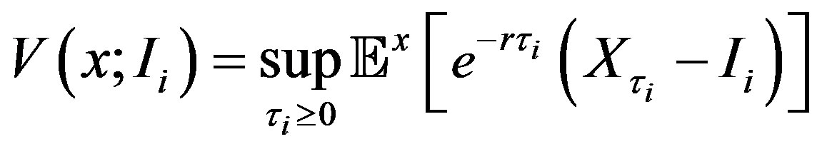 ,
,  , (2)
, (2)
where  denotes the expectation operator given that
 , and
, and  is the stopping time at which the investment is exercised once
  arrives at the threshold
  for
for , i.e.,
  Using standard arguments, the project value is rewritten as
 ,
, (3)
(3)
where . In this paper, the current state value
  is sufficiently low that the investment is not undertaken immediately.
The cash flow,  , is assumed to be observed by both the owner and the manager. However, the one-time cost,
  , is observed privately only by the manager.5 Immediately after making a contract with the owner at time zero, the manager observes whether the cost expenditure is of “lower cost” or “higher cost.” On the other hand, the owner cannot observe the true value of
 . Therefore, the owner must induce the manager to reveal private information truthfully at the time when the manager undertakes the investment. Otherwise, the owner suffers from further losses. Suppose, for example, the manager observes
  as the realized value of I. Then the manager diverts the difference
  to himself/herself by reporting
  to the owner. To prevent the diversion, the owner must encourage the manager to report the true value by providing incentives.
2.2. Asymmetric Information Problem
In this subsection, we formulate the owner’s maximization problem under asymmetric information. As explained earlier, under asymmetric information, the owner must induce the manager to reveal the manager’s private information truthfully.
In this paper, the owner designs a contract at time zero that commits the owner to give the incentive-disincentive to the manager at the time of investment. Renegotiation is not allowed. While commitment may cause ex post inefficiency in investment timing, it increases the ex ante owner’s option value. To reveal private information, we assume that the owner provides a bonus-incentive  and/or audits the manager with a probability
  at the time of investment.
The audit technology allows the owner at the cost to verify the state announced by the manager, and to impose a penalty on the manager for cheating when a false report is detected. We assume that a penalty  is an exogenous constant, and that the cost of auditing
  is a function of probability
  with
with ,
,  ,
,
 , and
, and . These assumptions are intuitively reasonable. The first assumption is that there is no cost incurred if the owner does not use the audit technology. The second and third assumptions imply that
  is strictly increasing and convex in
 . The final assumption is that complete auditing incurs a huge cost that the owner cannot pay.
Thus, the contract in the asymmetric information problem is modelled as a mechanism:6
 ,
, .
.
Let superscript “A” refer to the asymmetric information (agency) problem.7
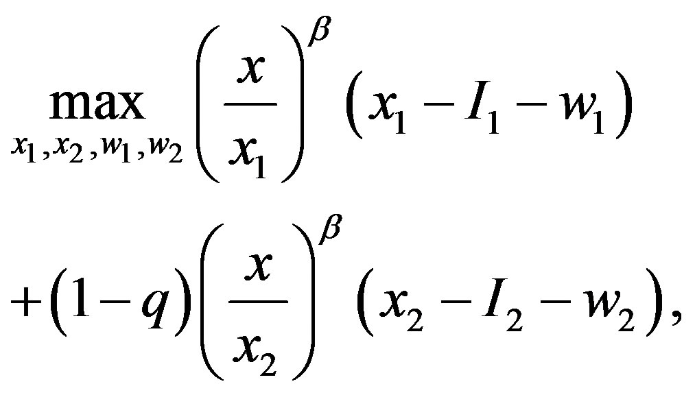
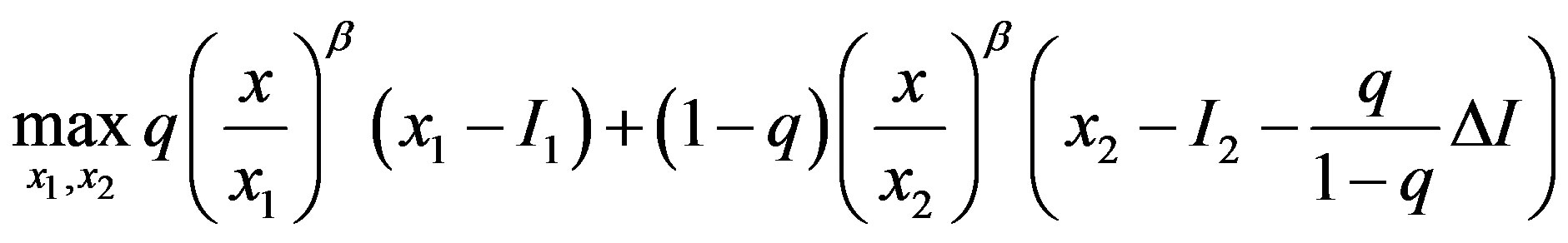
Then, the asymmetric information problem is to maximize the owner’s option value through choice of the mechanism , i.e.,
 (4)
(4)
subject to
 , (5)
, (5)
 , (6)
, (6)
 , (7)
, (7)
 ,
,  , (8)
, (8)
 ,
, . (9)
. (9)
Here, the objective function (4) is the ex ante owner’s option value.
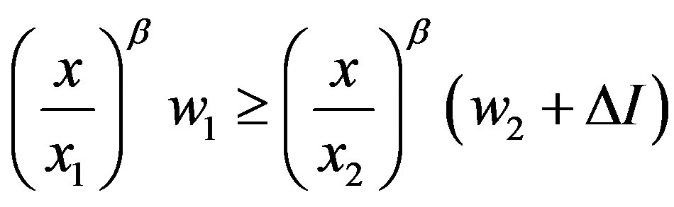
Constraints (5) and (6) are the ex post incentive-compatibility constraints for the manager under states  and
and , respectively. Consider, for example, constraint (5). The manager’s payoff in state
  is
is  if he/she tells the truth, but it is
  if he/she instead claims that it is state
 . Thus, he/she tells the truth if (5) is satisfied. Constraint (6) follows similarly. Constraint (6) will be shown not to be binding. Thus, only constraint (5) is relevant to our discussion.
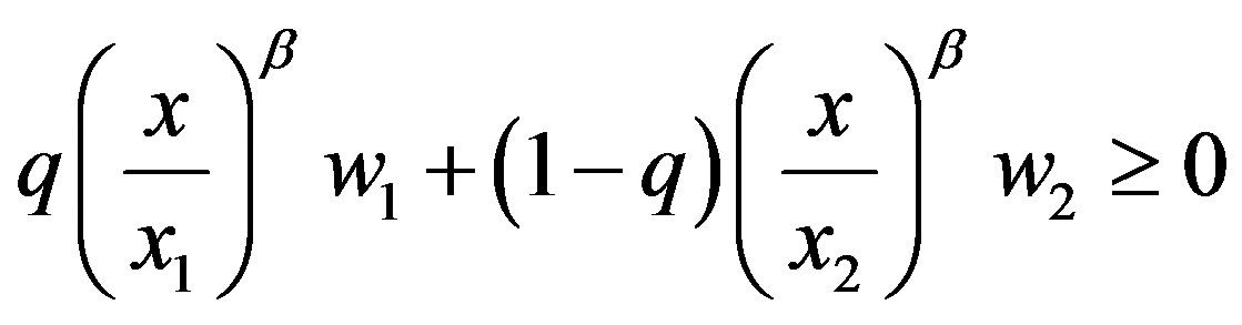
Constraints (7) and (8) are the ex ante participation constraint and the ex post limited-liability constraints, respectively. Constraints (8) ensure that the manager makes an agreement about employment. For example, if  , then the manager would refuse the contract on learning that
 . In addition, it is straightforward to show that constraint (8) implies constraint (7). Thus, only constraint
  will be relevant to our discussion.
Constraint (9) is obvious, where  is the probability of an audit.
Before analysing the asymmetric information problem, we first review briefly the symmetric information problem.
2.3. Symmetric Information Problem (Standard Real Options Model)
In this subsection, we consider the optimization problem when the owner observes the true value of . This problem is equivalent to the problem in which there is no delegation of the investment decision because the manager has no informational advantage. Then we have
  and
and  for all
  (
( ). Thus, the contract
  in the symmetric information problem is modelled as
 ,
, .
.
Let superscript “asterisk” refer to the symmetric information (no-agency) problem.
In the symmetric information case, the owner’s maximization problem is defined as
 (10)
(10)
where  (
( ). The solutions are
 . (11)
By substituting these solutions, we have
 (12)
(12)
We employ these results as a benchmark which is the same as those in the standard (MS) model.
3. Solution
In this section, we provide the solution to the asymmetric information problem that was described in the previous section. We then discuss some properties of the solution.
3.1. A Simplified Asymmetric Information Problem
Although the optimization problem is subject to seven inequality constraints, we can simplify the problem in the following three steps. In this subsection, we simplify the asymmetric information problem.
First, (7) is automatically satisfied, because (8) implies (7). Second, a manager in state  does not have the incentive to tell a lie as a manager in state
 , because the manager in state
  suffers a loss from such a false announcement. Thus, (6) is satisfied automatically, and
  and
and  are obtained at the optimum. Finally,
  in (9) is satisfied automatically. This statement is shown by
  and
and  for any
 .
.
As a result, the simplified optimization problem is given as
 (13)
(13)
subject to
 ,
,  ,
,  , (14)
where  for all
  (
( ).
).
3.2. Optimal Contracts
We first define the three feasible regions that serve to determine the characteristics of the solution. The nature of the solution depends on the magnitude of the penalty . The contract can be derived in three possible regions: the incentive-only (bonus-incentive only, Ab) region, the incentive-disincentive (combination, Ac) region, and the disincentive-only (audit-penalty only, Aa) region. Let superscripts “Ab”, “Ac”, and “Aa” refer to the optimums for the three feasible regions, respectively.
As shown in Appendix A, we can obtain the following results.
Proposition 1 Suppose that the penalty is finite. In the asymmetric information problem, the optimal contract  is as follows:
Incentive-only (bonus-only, Ab) region: 
 ,
,  where
where  and
and  are the investment trigger for
  and the bonus for
  in GW model as shown in Appendix B.
Incentive-disincentive (combination, Ac) region: 
 ,
,  where
where
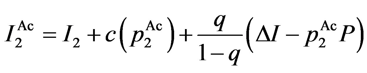 .
.
Disincentive-only (audit-only, Aa) region: 
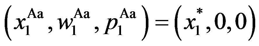 ,
,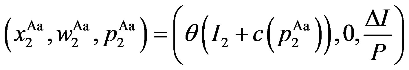 .
.
Here, in Region Ac,  is decided by
 , and
, and  is decided by
 . Similarly, in Region Aa,
  is decided by
 .
.
Note that, if the penalty is finite, the contracts under asymmetric information are significantly different from those under symmetric information. We then discuss the properties of the solution to the asymmetric information problem. Then, we have the following results (see Appendix A for the proof).
Corollary 1 Suppose that the penalty is finite. The optimal contract has the following properties:
for any  (
( ). In particular, we have
 ,
, .
.
Corollary 1 implies that there are five important properties. The first property of the solution is that  and
and  for any
 . It is less costly for the owner to distort
  away from
  than to distort
  away from
  in equilibrium.
The second property of the solution is that  and
and  if
if , and that
  and
and  otherwise. In other words, a decrease in
  is equivalent to the associated decrease in
 .
.
The third property of the solution is that  where
where  can be regarded as the information rent for the manager in state
 . The owner gives the manager in state
  a portion of the information rent. Importantly, note that the information rent is decreasing with
 .
.
The fourth property of the solution is that  is unimodal with
 . The reason is that
  is in-creasing and concave with
 , while
  is de-creasing and convex with
 . The first statement is straightforward because
  is increasing and convex with
 . The second statement is shown by
  at the optimum.
The final property of the solution is that an increase in the penalty  moves the contract
  from the incentive-only (Ab) region to the disincentive-only (Aa) region via the combination (Ac) region. This property is intuitive as follows. For example, the larger the penalty
  is, the more available the disincentive mechanism. Then, an increase in the penalty encourages the owner to use the disincentive mechanism rather than the incentive mechanism.
So far we have only considered the finite penalty. Now we examine the case of the unlimited penalty. Although the unlimited penalty is unrealistic, we are interested in considering how the contract changes as the penalty increases.
Recall that, under asymmetric information, there exists a distortion in three ( ,
,  ,
, ) of the six components of the contract, and that we have
 ,
,  ,
,  for
for . It is straightforward to show that
  as
as . Thus, these results are summarized as follows.
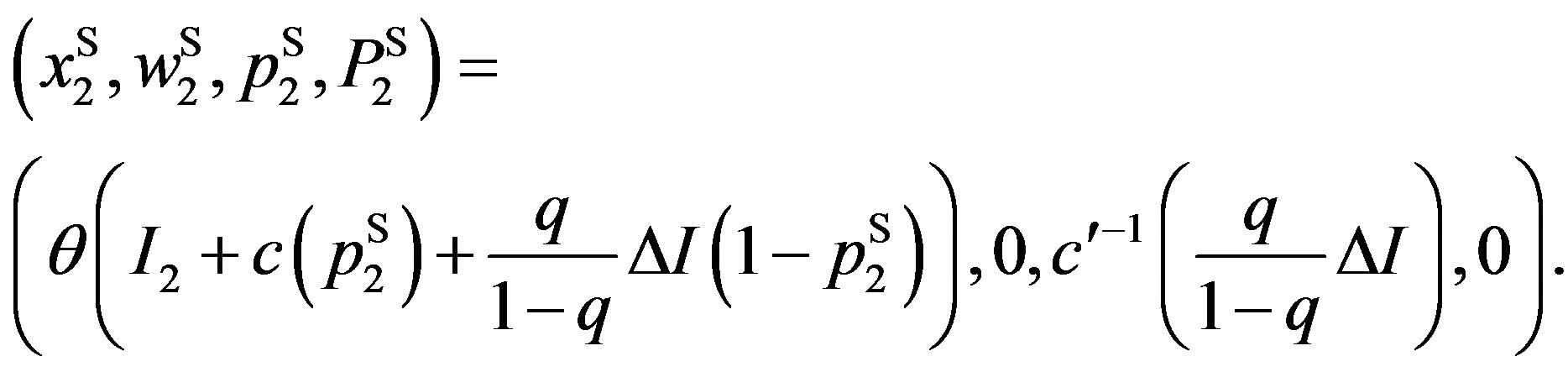
Corollary 2 The contracts under symmetric information are approximated closely as the penalty is increased without limit. As , we have
 ,
,  ,
, .
.
Recall that the solution in the symmetric information problem is the same as in the standard real options model. Thus, in contrast with previous papers under asymmetric information, we show that there is a relationship between the symmetric and asymmetric information problems. From Proposition 1 and Corollary 2, we have the following results.
Remark 1 The solution in the incentive-only (Ab) region is exactly the same as in the GW model. The solution for  in the combination (Ac) region turns out to be that in the S model. As the penalty
  becomes sufficiently large, the solution in the disincentive-only region in the asymmetric information model converges to in the symmetric information model developed by MS.
The first statement is obvious in Proposition 1. As for the second statement,  is endogenously decided in the S model as shown in Appendix B. Thus, we have the second statement from Proposition 1. The third statement is given by Corollary 2. As a result, Remarks 1 implies that the solutions in our model include those in the three related papers.
3.3. Optimal Values
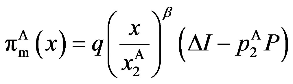
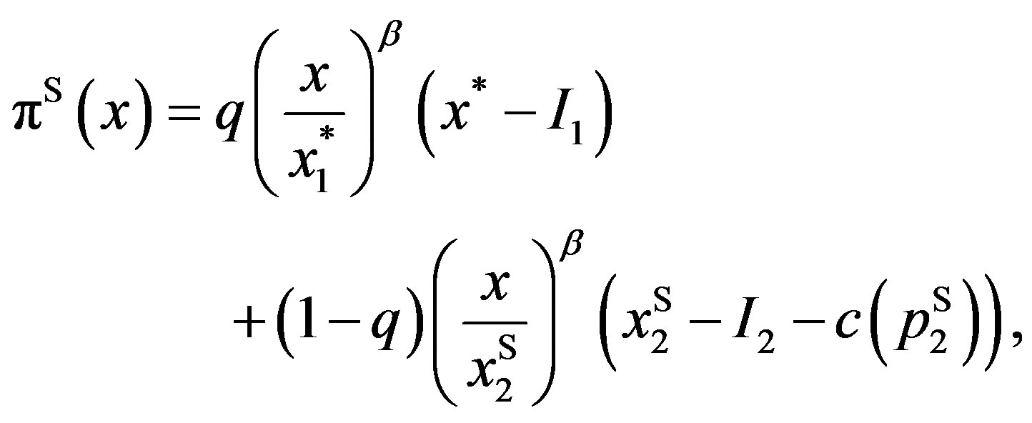
For all three feasible regions, substituting the solutions into the owner’s and manager’s option values,  and
and , respectively, yields
 (15)
(15)
where
and
 (16)
(16)
Because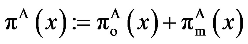 , the total value
  is
is
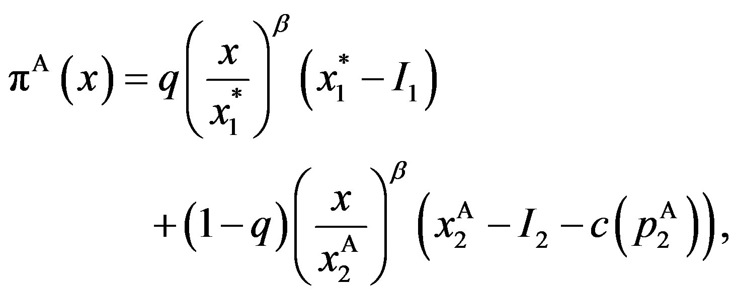 (17)
(17)
for any 
 . Obviously, inefficiency is caused by the second term in state
 .
.
Let us define ,
,  , and
, and  as the owner’s, manager’s, and total values in the GW model, as shown in Appendix B. Then, we obtain the following results.
Corollary 3 Suppose that the penalty is finite. Then we have
 ,
, .
.
In particular, the optimal value has the following properties:
 ,
, .
.
Moreover, we obtain
 ,
, .
.
Corollary 3 implies that there are three important properties. The first is that  is monotonically increasing in
 , while
  is monotonically decreasing in
 . The second is that asymmetric information always leads to a decrease in total value for any finite penalty
 . The third is that we do not always have
  although we always have
  . In summary, because the set of the incentive-disincentive contracts is enlarged by that of the incentive-only contracts in the GW model, the owner’s (manager’s) value is always larger (smaller) than in the GW model. However, the sum of these values is not always larger than in the GW model. Thus, depending on the parameters, we have
 . These imply that the owner’s rationality does not correspond to the total rationality. We will discuss this result in the next section by using numerical calculations.
In order to measure the “inefficiency” arising from asymmetric information, we define total social loss  as
as
 .
.
Here,  is strictly positive for any finite penalty P. This definition is exactly the same as in Subsection 4.3 of the GW model. We define the total social loss in the GW model as
 . Obviously from the definition, the properties of total value
  are equivalent to that of total social loss
 .8
.8
As the same as in the contracts, if the penalty  is sufficiently large, the following results are obtained.
Corollary 4 The values under symmetric information are approximated closely as the penalty is increased without limit. As , we have
 ,
,  ,
,  and
and
 .
.
The owner’s and manager’s values are monotonic with the penalty . In particular, the owner’s value is increasing monotonically in
 . However, the total value (i.e., total social loss) is non-monotonic with
 .
.
4. Numerical Implications
This section analyses several of the more important implications of the model by using the numerical examples. Subsection 4.1 investigates the effects of the exogenous maximum penalty on the solutions and values. Subsection 4.2 examines the distortion in asymmetric information, by using the total social loss. Subsection 4.3 examines the stock price reaction to the information released via the manager’s investment decision.
In the numerical examples, we define the auditing cost function  as
as
 ,
, (18)
(18)
Here, the parameter  is interpreted as a measure of “efficiency” for the auditing cost function. Assume that the basic parameters are
 ,
,  ,
,  ,
,  ,
,  ,
,  ,
,  and
and .
.
4.1. Effects of the Penalties
This subsection considers the effects of the penalties shown in Figure 1.
Under , the incentive-only (Ab) region is
  , the combination (Ac) region is
  , and the disincentive-only (Aa) region is
 . First of all, recall that the contracts in the GW model are the incentive-only contracts. The contracts in the incentive-only (Ab) region are the same as those in the GW model because
  for
for  (
( ). Next, note that the penalty is equal endogenously to the managers’ diverted cash flow, i.e.,
  . The contract for
  in the combination region turns out to be the same as that in the S model. Finally, as
 , the contracts in the disincentiveonly (Aa) region converge to the symmetric information contracts in the MS model.
The upper left-hand side panel of Figure 1 depicts the investment trigger  with respect to the penalty
  (
( ). We see that
  is decreasing mo-
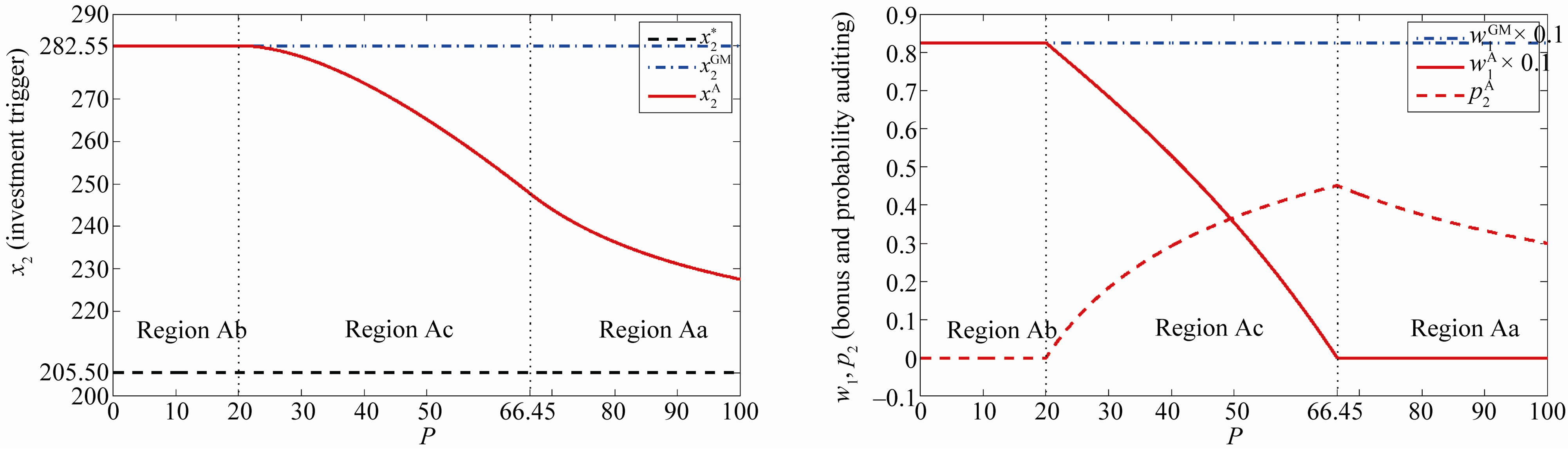
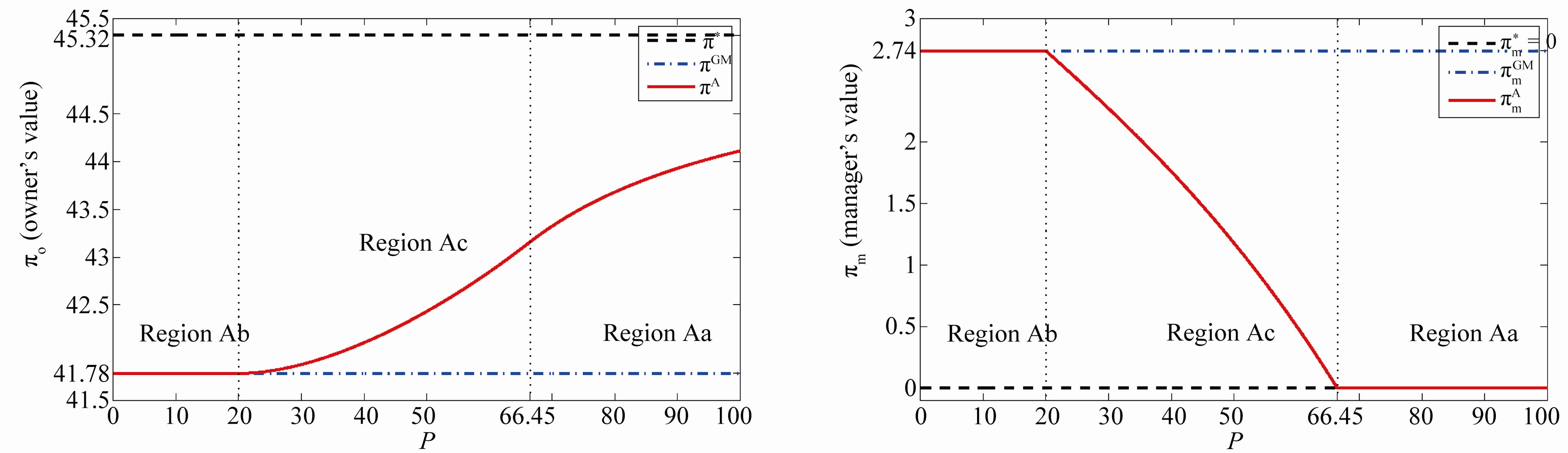
Figure 1. The effects of penalty. This figure illustrates the effects of the penalty on the investment trigger (upper left-hand side panel) the bonus and probability of an audit (upper right-hand side panel), owner’s value (lower left-hand side panel), and manager’s values (lower right-hand side panel). The incentive-only (bonus-only, Ab) region is 0 ≤ P ≤ 20, the combination (Ac) region is 20 ≤ P ≤ 66.45, and the disincentive-only (audit-only, Aa) region is P > 66.45.
notonically in  with
with .
.
The upper right-hand side panel demonstrates the bonus incentive and the probability of auditing,  and
and , with respect to
 . On the one hand,
  is decreasing with
  although
  is constant with
 . On the other hand,
  is unimodal with
 . In particular, as explained earlier,
  is increasing and concave with
 , while
  is decreasing and convex with
 .
.
The lower right-hand side panel depicts the owner’s option values  and
and  with respect to
 . The important result is that
  is in between two values,
  and
and . In addition,
  is increasing monotonically with
 . This property corresponds to the “maximal penalty principle” in the microeconomics literature.9
The lower right-hand side panel demonstrates the manager’s option values  and
and  with respect to
 . Recall that the manager’s value is zero under symmetric information while it is strictly positive constant under the GW model. The value
  is decreasing monotonically with
 . The reason is that an increase in
  decreases the information rent for the manager in state
 , which leads to the decrease in the bo-nus-incentive.
The upper right-hand and lower left-hand side panels imply that an increase in P leads to “asset substitution” between the owner and the manager. Wealth is transferred from the manager to the owner by an increase in P.
4.2. Distortion in Asymmetric Information
This subsection examines the distortion in the social welfare arising from the asymmetric information.
Figure 2 depicts the total social losses  and
and  with respect to
 . The most interesting result is that
  is not decreasing monotonically with
  although
  is constant with P. Here,
  is constant with
  because it is exactly the same as
 , while
  is always decreasing with
 . On the other hand,
  is increasing or decreasing with
 . Thus, an increase in
  does not necessarily lead to a decrease in
  although it always increases the owner’s option value. Consequently, an owner’s (individual) rationality does not necessarily lead to total social rationality.
In addition, we consider the comparative statics with respect to  (
( ). Under
 , Region Ab is
 , Region Ac is
 , and Region Aa is
 . Under
 , Region Ab is
 , Region Ac is
 , and Region Aa is
 . An decrease in the parameter
  does not necessarily decrease
 . Consider, for example,
 . Then,
  under
under  is smaller than under
 . Thus, a reduction in the inefficiency of the auditing cost always benefits the owner, while it does not necessarily increase total social welfare.
4.3. Stock Price Reaction to Investment
This subsection investigates the stock price reaction to the manager’s investment decision. The stock price is the owner’s option value that is given in (15).
Prior to the point at which  reaches the trigger
 , the market does not know the true value of
 . The market believes that
  with probability
  and
and  with probability
 .
.
Once x hits the trigger , the private information is fully revealed. The manager’s investment decision signals
  to the market. If the manager undertakes the investment at
  , then the stock price instantly jumps upwards to
 ,
, .
.
Thus, the jump size in the stock price is  where
where
Otherwise, the market assumes . Then the stock price instantly jumps downwards to
 .
.
The side of the downwards jump is  . Thus, the sizes of upwards and downwards jumps are the same under
 .
.
The upper left-hand side panel of Figure 3 demonstrates the stock price reaction to investment. Here, we generate stock price paths computed with the same parameters as in the previous section and fixed . Then the stock price is 63.42 just prior to
  . If the manager undertakes the investment at
 , the stock price jumps upwards to 73.13. Otherwise, the stock price jumps downwards to 53.70. Thus, the jump size in the stock price reaction to investment is 9.71 under
 .10
.10
We begin by investigating the effect of the penalty  on the size of the stock price reaction to investment. Consider a change in the penalty
  from 0 to 100. Our intuitive conjecture is as follows. The jump size in the stock price reaction is decreasing monotonically in P

Figure 2. Total social loss with respect to penalty. The total social loss LA(x) is non-monotonic with P. In addition, LA(x) is not necessarily decreasing with α. Under α = 1, Region Ab is 0 ≤ P ≤ 1, Region Ac is 1 ≤ P ≤ 36, and Region Aa is P ≥ 36. Under α = 5, Region Ab is 0 ≤ P ≤ 5, Region Ac is 5 ≤ P ≤ 45, and Region Aa is P ≥ 45.
because the difference in the stock prices between the symmetric and asymmetric information problems is decreasing monotonically in the exogenous penalty , shown in the left-hand side panel of Figure 1. Interestingly, however, contrary to our intuitive conjecture, the jump size in the stock price reaction need not be monotonic in
 , shown in the upper right-hand side panel of Figure 3. The reason is that
  is non-monotonic with P. This result is also new and not shown by the GW model where
 . Note that the jump size in the GW model corresponds to that in the incentive-only region (
 ) in our model.
Therefore, in contrast to our intuition, the jump size in the stock price reaction to investment has a Λ-shaped relation with .
.
Next, we examine the effect of the volatility parameter , shown in the lower right-hand side panel. The volatility parameter
  is changed from 0 to 0.4. The other parameters are unchanged. We see that the jump size in our model and the GW model are 9.71 and 7.24 under
 , respectively. Here interestingly, the jump size in our model is increasing in
 , while in Grenadier and Wang [2] it is decreasing in
 . The reason is that the probability is a Λ-shaped curve with
 .
.
Finally, we examine the effect of efficiency measure  on the auditing cost function, shown in the lower right-hand side panel. The efficiency measure
  for the auditing cost function is changed from 10 to 40. Again, contrary to our intuition, the jump size in the stock price reaction to investment is decreasing in
 .
.
5. Concluding Remarks
Our paper extended the investment timing decision problem under asymmetric information by adopting the enlarged set of incentive-disincentive contracts framework. Investment timing under asymmetric information is delayed, compared with that under asymmetric information. However, investment timing under asymmetric information converges to the symmetric information investment timing by making the disincentive (penalty) for the manager’s untruthful report sufficiently large. Consequently, by adopting the enlarged set of incentive-disincentive contracts framework, we showed that there is a relationship between the symmetric and asymmetric information problems.
We consider the inefficiency in the social welfare under the enlarged set of incentive-disincentive contracts. Based on the fact that the investment timing and stock price (owners’ value) in our model are between those of MS and GW, we conjecture intuitively that social welfare
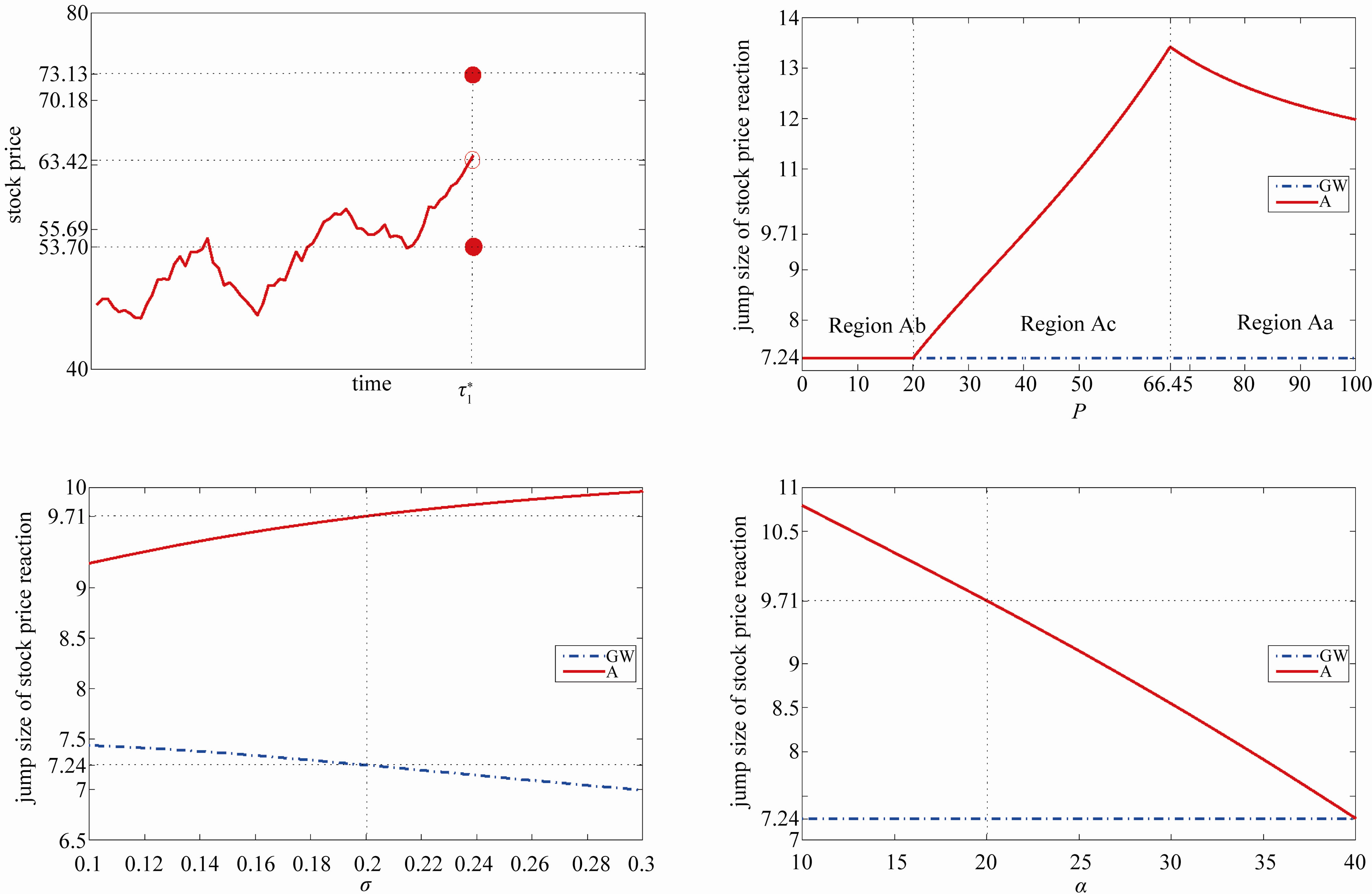
Figure 3. Jump size of stock price reaction to investment. The upper left-hand side panel plots the sample path of the stock price under P = 40. Once Xt arrives at , the private information is fully revealed. The stock price is 63.42 just prior to
 . If the manager adopts the investment at
 , then this action signals I = I1 to the market. Thus, the stock price jumps upwards to 73.13. Otherwise, the stock price jumps downwards to 53.70. The jump size is 9.71 under P = 40. The upper right-hand side panel illustrates the jump size of the stock price reaction to investment for various values of P. The jump size has a Λ-shaped relation with P. The lower left-hand side panel depicts the effects of jump size with respect to the volatility. The lower right-hand side panel demonstrate the jump size of the efficiency measure for the auditing cost function.
in our model is also between social welfare in those two papers. However, the result is not necessarily correct. We showed that owners’ rationality does not necessarily lead to total social rationality.
REFERENCES
- A. Dixit and R. S. Pindyck, “Investment under uncertainty,” Princeton University Press, Princeton, 1994.
- S. R. Grenadier and N. Wang, “Investment Timing, Agency, and Information,” Journal of Financial Economics, Vol. 75, No. 3, 2005, pp. 493-533. doi:10.1016/j.jfineco.2004.02.004
- H. Weeds, “Strategic Delay in a Real Options Model of R & D Competition,” Review of Economic Studies, Vol. 69, No. 3, 2002, pp. 729-747. doi:10.1111/1467-937X.t01-1-00029
- M. Nishihara and M. Fukushima, “Evaluation of Firm’s Loss Due to Incomplete Information in Real Investment Decision,” European Journal of Operational Research, vol. 188, No. 2, 2008, pp. 569-585. doi:10.1016/j.ejor.2007.03.046
- A. E. Bernardo and B. Chowdhry. “Resouces, Real Options, and Corporate Strategy,” Journal of Financial Economics, Vol. 63, No. 2, 2002, pp. 211-234. doi:10.1016/S0304-405X(01)00094-0
- T. Shibata, “The Impacts of Uncertainties in a Real Options Model under Incomplete Information,” European Journal of Operational Research, Vol. 187, No. 3, 2008, pp. 1368-1379. doi:10.1016/j.ejor.2006.09.019
- A. Mello and J. J. Parsons, “Measuring the Agency Costs of Debt,” Journal of Finance, Vol. 47, No. 5, 1992, pp. 1887-1904. doi:10.2307/2329000
- H. E. Leland, “Agency Costs, Risk Management, and Capital Structure,” Journal of Finance, Vol. 53, No. 4, 1998, pp. 1213-1243. doi:10.1111/0022-1082.00051
- R. Townsend, “Optimal Contracts and Competitive Markets with Costly State Verification,” Journal of Economic Theory, Vol. 33, 1979, pp. 265-293. doi:10.1016/0022-0531(79)90031-0
- D. Baron and D. Besanko, “Regulation, Asymmetric Information, and Auditing,” RAND Journal of Economics, Vol. 15, No. 4, 1984, pp. 447-470. doi: 10.2307/2555518
- J. J. Laffont and J. Tirole, “Using Cost Observation to Regulated Firms,” Journal of Political Economy, Vol. 94, No. 3, 1986, pp. 614-641. doi:10.1086/261392
- T. Shibata, “Investment Timing, Asymmetric Information, and Audit Structure: A Real Options Framework,” Journal of Economic Dynamics and Control, Vol. 33, No. 4, 2009, pp. 903-921. doi:10.1016/j.jedc.2008.10.005
- R. McDonald and D. R. Siegel, “The Value of Waiting to Invest,” Quarterly Journal of Economics, Vol. 101, No. 4, 1986, pp. 707-727. doi:10.2307/1884175
- D. Fudenberg and J. J. Tirole, “Game theory,” MIT Press, Cambridge, 1991.
- J. J. Laffont and D. Martimort, “The Theory of Incentives: The Principal-Agent Model,” Princeton University Press, Princeton, 2002.
Appendix A. Proof of Lemma and Proposition
A.1. Proof of Proposition 1
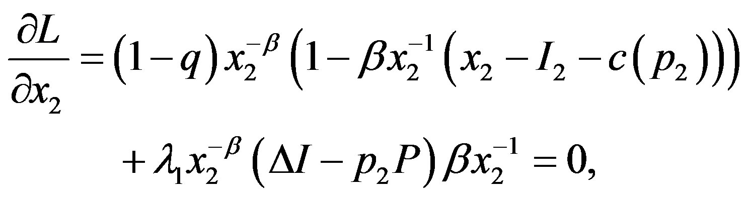
By omitting , the Lagrangian can be formulated as:
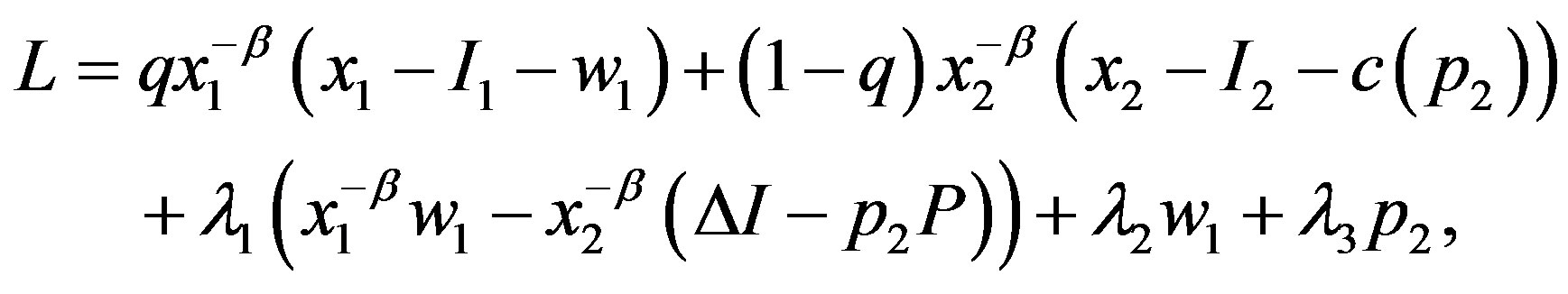
where  (
( ) denotes the multiplier on the constraints. The Kuhn-Turker conditions are
 ,
, 
 ,
,  ,
,  and
and
 ,
,  ,
, .
.
The solution depends on whether or not  and
and  are equal to zero. First, suppose that
  and
and . Then we have
  and
and  implying
 , which contradicts
 . Thus, at least one of
  and
and  must be binding. Second, suppose that
  and
and . Then since
 , we have the solution in the bonus-only (Ab) region with
 . Third, suppose that
 . Then we obtain
  and
and . It is straightforward to obtain the solution in the combination (Ac) region. Finally, suppose that
  and
and . Then we have
  , and
, and  because of
  . Thus, we get the solution in the auditonly (Aa) region with
  .
.
A.2. Proof of Corollary 1
Here, we prove that . First, it is easy to obtain
  from
from
 and
and . Second,
  can be proved because of
 and
and . Finally, we prove
 . The trigger
  is equal to
 .
.
Here, we have used  at the optimum. Because
  is strictly increasing and convex with
 , the second term is negative. Thus, the proof is complete.
Appendix B. Related Papers
This appendix explores the two problems in GW and S.
B.1. Grenadier and Wang (GW) Model
The GW model (asymmetric information problem with the incentive-only mechanism) is formulated as:
subject to
 ,
,  ,
,  ,
,  ,
, .
.
At the optimum, we can simplify the problem as follows:
 . (B.1)
Equation (B.1) means that the owner’s value is reduced by the term , compared with the symmetric information problem defined by (10). The optimal contracts are obtained by
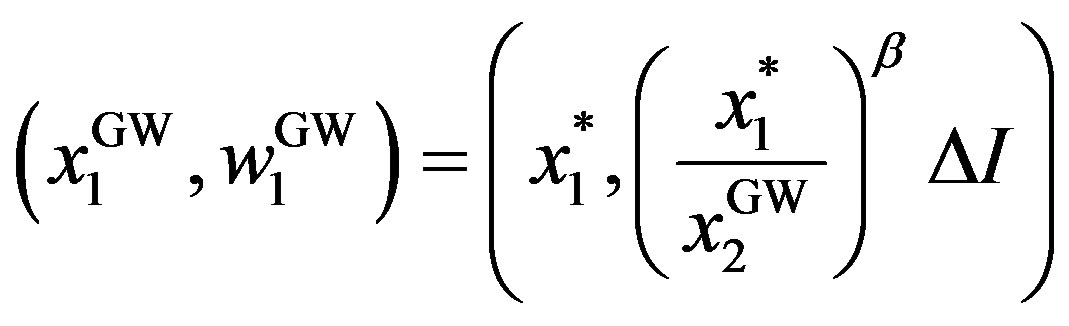 ,
,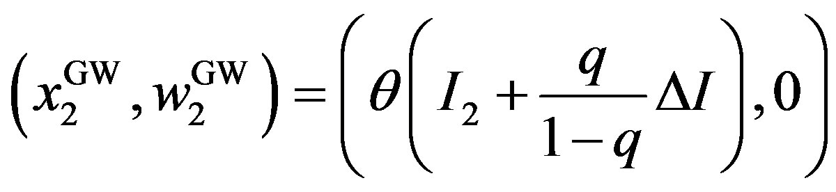 .
.
The superscript “GW” refers to the optimum in the GW model. The owner’s, manager’s, total values are given as
 ,
,  where
where .
.
B.2. Shibata (S) Model
The Shibata model (asymmetric information problem with the incentive-disincentive mechanism with limitedliability constraints on penalties) is defined by:

subject to
 ,
,  ,
,  ,
,  ,
,  ,
,  ,
,  ,
,  ,
, .
.
Then, we obtain ,
,  ,
,  and
and  where the superscript “S” refers to the optimum in the S model, and reduce the number of constraints to only one:
 (B.2)
(B.2)
subject to . Equation (B.2) is reduced by the term
 , compared with (10) in the symmetric information problem. The optimal contracts are obtained as follows. If
 ,
,  turns out to be:
 ,
, 
Otherwise, the solutions are equal to those in which  is substituted. The owner’s, manager’s, and total values become

 ,
, 
where .
.
NOTES
*This research was partially supported by a Grant-in-Aid by the Excellent Young Researcher Overseas Visit Program (21-2171), the Japan Economic Research Foundation, KAKENHI (22710142, 22710146), the Telecommunications Advancement Foundation, the Zengin Foundation for Studies and Economics and Finance.
1Recently, the standard real options model has been extended in various ways. For example, Weeds [3] and Nishihara and Fukushima [4] consider investment timing by taking into account strategic interactions. Bernardo and Chowdhry [5] and Shibata [6] analyse investment decisions under incomplete information.
2While these papers focus on the agency conflicts between owners and managers, a similar problem exists between stockholders and bondholders. Mello and Parsons [7] and Leland [8] examine the agency problem between stockholders and bondholders using the real options approach.
3See Townsend [9], Baron and Besanko [10], and Laffont and Tirole [11].
4The assumption r > μ is needed to ensure that the value of the firm is finite.
5The assumption that a portion of the project value is observed privately only by one person (here, the manager) and not observed by the other (here, the owner) is quite common in the asymmetric information litrature. An excellent overview of the analysis of asymmetric information situations is found in Fudenberg and Tirole [14] and Laffont and Martimort [15].
6We need not examine the possibility of a pooling equilibrium. This is because a pooling equilibrium is always dominated by a separating equilibrium.
7Because at the equilibrium the manager reveals truthfully the true Ii as private information, we make no distinction between the reported  and the true Ii.
8We will discuss LA(x) rather than πA(x) when we investigate inefficiency in social welfare.
9See Laffont and Martimort [15] for details.
10In the incentive-only contracts in the GW model, the stock price jumps from 62.93 upwards and downwards to 70.18 and 55.69, respectively. The jump size is 7.24.