Journal of Electromagnetic Analysis and Applications
Vol. 3 No. 12 (2011) , Article ID: 16520 , 10 pages DOI:10.4236/jemaa.2011.312079
Characterization of an Electromagnetic Vibration Isolator
![]()
Department of Mechanical Engineering, Lakehead University, Thunder Bay, Canada.
E-mail: kliu@lakeheadu.ca
Received October 25th, 2011; revised November 22nd, 2011; accepted November 30th, 2011.
Keywords: High-static-low-dynamic stiffness spring, semi-active vibration isolator, magnetic spring, coupling of structural mechanics and magnetics
ABSTRACT
A novel vibration isolator is constructed by connecting a mechanical spring in parallel with a magnetic spring in order to achieve the property of high-static-low-dynamic stiffness (HSLDS). The HSLDS property of the isolator can be tuned off-line or on-line. This study focuses on the characterization of the isolator using a finite element based package. Firstly using the single physics solver, the stiffness behaviours of the mechanical and magnetic springs are determined, respectively. Then using the weakly coupled multi-physics method, the stiffness behaviours of the passive isolator and the semi-active isolator are investigated, respectively. With the found stiffness models, a nonlinear differential equation governing the dynamics of the isolator is solved using the time-dependent solver. The displacement transmissibility ratios of the isolator are obtained. The study confirms that the isolation region of the isolator can be widened through off-line or on-line tuning.
1. Introduction
Vibration isolation is one of the vibration suppression methods [1-5]. There are two kinds of vibration isolation: to isolate a vibration source from its support and to isolate a base excitation from a device. This study focuses on the second type. A simplest vibration isolator consists of a spring and a damper arranged in parallel. The spring plays a dual role: to support the weight of the device and to isolate the base motion. For a linear spring isolator, vibration isolation occurs when the natural frequency ωn of the isolator system is smaller than  where ωb is the frequency of the base motion or exciting frequency. To increase the isolation region, the stiffness of the isolator spring should be made as low as possible. However, lowering the isolator’s stiffness results in a large static deflection that is undesirable. To overcome this problem, a high-static-low-dynamic stiffness (HSLDS) spring can be used. The HSLDS isolator is capable of supporting a large static load while possessing a low natural frequency [6,7].
A passive isolator is effective if operating conditions remain unchanged. However, if operating conditions vary, the isolator’s performance may deteriorate. A semiactive or tunable vibration isolator is capable of altering its stiffness or damping level in real time based on the response. Semi-active vibration isolators have been receiving increasing interest because they combine the advantages of both the passive and active devices [8-10]. On one hand, they preserve the reliability of the passive devices even in the event of power loss; on the other hand, they possess the adaptability of the active devices without a great amount of power consumption.
The tunable HSLDS isolator proposed in [11,12] belongs to the family of variable stiffness devices. The notable feature of the device is that its stiffness can be instantly decreased or increased without any moving parts. The ability of on-line tuning makes the isolator quickly adapt to the operating conditions so that the optimal performance is maintained. The isolator spring consists of a mechanical spring and an electromagnetic spring. As both the springs are nonlinear, determination of their stiffness models presents a challenge. In [11,12] an experimental approach was taken for this purpose. Another effective method to deal with such a system that involves two physics is to use a finite element (FE) based multiphysics software. This paper reports a characterization study for the isolator using Comsol Multiphysics, a commercial FE package. The aim of the study is twofold: to determine the stiffness behaviors of the isolator springs, and to evaluate the performance of the isolator in a passive mode or semi-active mode. The rest of the paper is organized as follows. In Section 2, the proposed HSLDS isolator is introduced. In Section 3, the stiffness characterization is addressed. In Section 4 the displacement transmissibility of the HSLDS isolator is evaluated. In Section 5, the study conclusions are presented.
2. A Tunable HSLDS Isolator
Figure 1 shows a schematic of the tunable HSLDS isolator proposed in [11,12]. A steel beam (2) is used to support a permanent magnet (PM) (3). The permanent magnet acts as an isolated mass and is referred to as mass m. The mass-beam assembly is placed between a pair of electromagnets (EMs) (4). The EMs are fastened to an aluminum base through two aluminum brackets. The mass-beam assembly is held by two aluminum supports (1) that are fixed onto the base. The tension of the beam can be adjusted by the screws (5). The EM coils are constructed by Gauge 22 copper wire. The outer diameter and length of the coil are 46.6 mm and 88.0 mm, respectively. The number of the coil turns is about 3565. The EM core is a low-carbon steel bolt with a diameter of 13.0 mm and length of 150.0 mm.
As shown in Figure 2, two springs are involved in the isolator. The beam acts as a mechanical spring denoted as kb. The interaction between the PM and the EMs results in an electromagnetic spring denoted as kpe. The electromagnetic spring kpe consists of two parts: kpc and kpf where kpc is due to the interaction between the PM and the EM cores and kpf is due to the interaction between the PM and the flux generated by the EMs. Note that the net magnetic force acting on the mass or PM behaves in the following way. When the mass is located exactly in the middle of the gap of the EMs, the net magnetic force is zero. With the EM polarities shown in Figure 2, when
Figure 1. Schematic of the tunable HSLDS isolator.
Figure 2. Two springs involved in the proposed isolator.
the mass moves to the left, the net magnetic force acts leftward, which corresponds to a negative magnetic stiffness. With the reversed EM polarities, when the mass moves to the left, the net magnetic force acts rightward, which corresponds to a positive magnetic stiffness. It should also be noted that the static stiffness depends only on the mechanical spring, while the dynamic stiffness comes from the combined effect of the mechanical spring and the electromagnetic spring.
3. Stiffness Characterization
3.1. The Mechanical Spring
Figure 3 illustrates the Comsol model used to study the stiffness of the mechanical spring. The model was created in the Plane Stress mode of Structural Mechanics module. A 2-D model is used in order to reduce computational burden. The mass or PM is represented by block (3) with a size of 25.4 × 29.0 mm (width × height). The beam is represented by member (2) with a size of 148.0 × 0.5 mm (length × thickness) and a Young’s modulus of 207.0 GPa. To account for the effect of the beam supports, two vertical aluminum beam members (1), with their ends fixed, are used. The size of the vertical aluminum beams is 80.0 × 3.0 mm (length × thickness) and the Young’s modulus is 70.0 GPa. The depth of all the members is 25.4 mm.
To find the stiffness of the mechanical spring, a vertical force is applied to the center of the mass. Using the parametric solver, the displacements of the mass corresponding to a given range of the vertical forces are obtained. The solid line in Figure 4 represents the relationship between the applied force and the mass displacement. From this relationship, the stiffness of the mechanical spring can be found. To verify the Comsol simulation result, an experiment was conducted to determine the relationship between the applied force and mass displacement [12]. The circles in Figure 4 represent the experimental values. It can be seen that the two results agree each other. Figure 5 compares the stiffness
Figure 3. Comsol model of the mass-beam-support assembly.
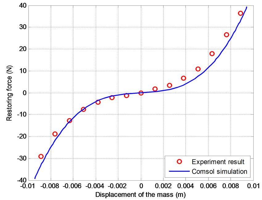
Figure 4. Restoring force of the mechanical spring versus the mass displacement.
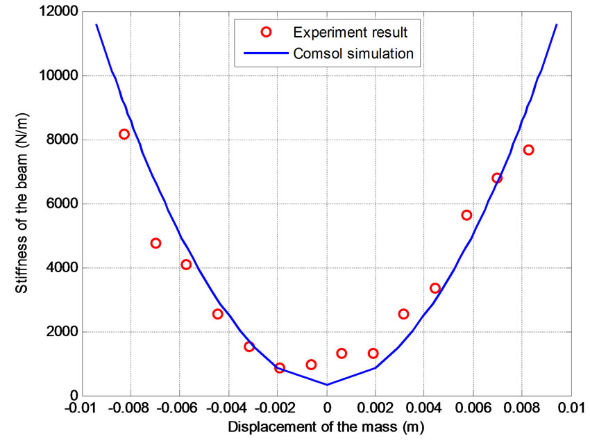
Figure 5. Stiffness of the mechanical spring.
values computed from the force-displacement relationships. It is noted that the stiffness increases with an increase of the mass displacement. This indicates that the mechanical spring exhibits the characteristics of a hardening spring.
3.2. The Electromagnet Spring
Figure 6 shows the Comsol model for the electromagnetic spring the model is built using Magnetostatics mode of AC/DC Module. The PM is modeled as a block with a size of 25.4 × 25.4 × 29.0 mm (length × width × height). The magnetization of the PM is 786.23 k·Am−1. Each of the EMs is modeled as an assembly of a solid cylinder representing the steel core and a hollow cylinder representing the coil. The diameter and length of the solid cylinder are 13.0 mm and 150.0 mm, respectively. Its relative permeability is 152.7 when the EM current is zero. The inner and outer diameters of the hollow cylinder are 13.0 mm and 46.6 mm, respectively. The length of the hollow cylinder is 88.0 mm. The EM-PM-EM assembly is surrounded by two cylindrical free spaces. The dimension of the inner free space is 660.0 × 160.0 mm (length × diameter) and the dimension of the outer free space is 700.0 × 200.0 mm (length × diameter). The outer free space consists of infinite elements [13].
Magnetic force simulations require a fine mesh in order to obtain a reasonable accuracy. In particular, the mesh on the exterior boundaries of the object where the force is evaluated needs to be extra fine. A finer mesh reduces the computation error but consumes more computer resources. The “Normal” mesh was used in the model. In order to ensure an accurate evaluation of the force, the maximum element size is specified for the relevant members. In particular, the maximum element size of the two hollow cylinders is 4.0 mm. The maximum element size of the two pole faces of the PM and the adjacent end faces of the steel cores is 1.0 mm.
The magnitude of the external current density that flows in the cross section of the hollow cylinder is approximated to be the EM current density in each turn.
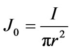 (1)
(1)
where J0 is the magnitude of the external current density, I is the current in the EM and r is the radius of the coil wire. The x component of the external current density is (the coordinate system is defined in Figure 6)
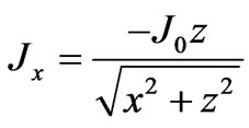 (2)
(2)
and the z component of the external current density is
 (3)
(3)
When the PM is placed between the EMs that are not energized, the interaction between the PM and the steel cores of the EMs constitutes a permanent magnet spring. When the PM is in the middle of the gap of the EMs, the net force on the PM is zero. When the PM is displaced along the y axis, the net force tends to move the PM away from its equilibrium position. Such a force is considered to be a negative restoring force. By placing the PM at different locations along the y axis, the relation
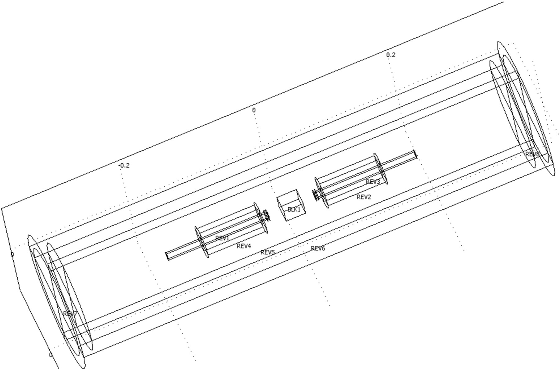
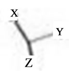
Figure 6. Comsol model of the electromagnetic spring.
ship between the net force and the PM displacement is obtained. Figure 7 presents the force-displacement curves for four different gap distances. From these relationships, the stiffness relationships are obtained. Figure 8 shows the stiffness curves of the PM spring corresponding to the results of Figure 7. It can be observed that when the gap distance becomes smaller, the stiffness becomes more negative. In addition, the greater the gap distance, the smaller the stiffness variation.
When the EMs are energized, the force acting on the PM depends on several factors such as the flux density produced by the EMs, the magnetization and position of the PM, and the relative permeability and size of the steel cores. Many studies have shown that the relative permeability of ferromagnetic materials is sensitive to several factors such as temperature and applied magnetic field intensity [14-16]. For example, when an electromagnet is energized, the temperature of its core will rise, which inevitably alters the relative permeability of the core. And when a PM is near a ferromagnetic material, the strong magnetic field generated by the PM will lower the relative permeability of the material. Therefore, selecting a proper relative permeability for the steel core plays a critical role in simulation.
In this study, to simplify the simulation, it is assumed that the relative permeability of the steel core depends only on the amplitude of the EM current. To obtain proper relative permeability values, the following approach was taken. First an experiment was conducted to measure the interacting forces between the PM and one EM. After a DC current was applied to the EM, the forces acting on the PM were measured for different gap distances between the PM and the EM. The circles in Figure 9 are the measured force values corresponding to the EM currents varying from −2.0 A to 2.0 A at the step size of 0.2 A. Then in order to compute the interacting force between the PM and one EM, one of the EMs in the model shown in Figure 6 was removed. Using a trial value for relative permeability, the force between the PM and the EM was computed for a given EM current and gap distance. By varying the gap distance from 2.0 mm to 60.0 mm at the step size of 2.0 mm and fixing a cur-
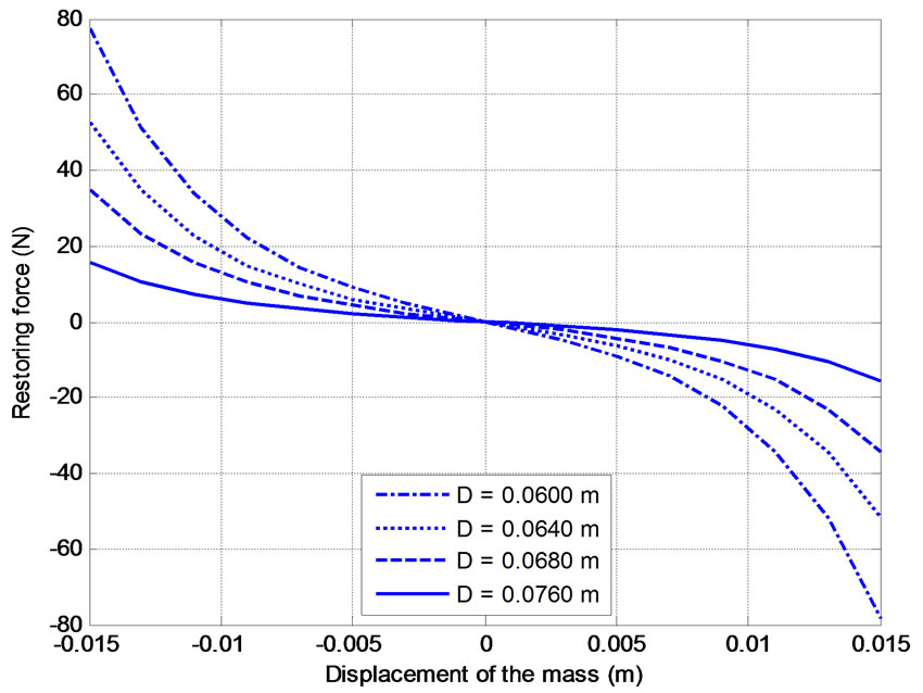
Figure 7. The net force on the PM for four different gap distances.
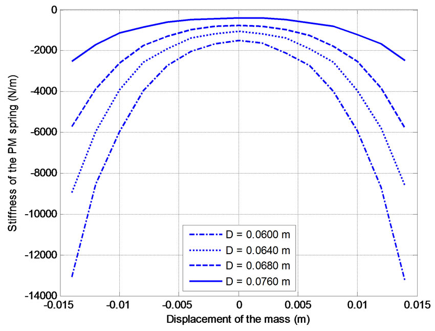
Figure 8. Stiffness of the permanent magnet spring for four different gap distances.
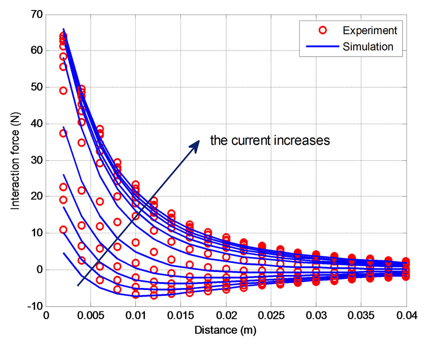
Figure 9. Interacting forces between the PM and the EM when the currents vary from −2.0 A to 2.0 A in a step of 0.4 A.
rent, the relationship between the computed force and the gap distance was obtained. The root-means-squared (RMS) error between the computed force values and the measured ones for a given current was found. Varying the relative permeability value changed this RMS error. The simulation was repeated by varying the relative permeability values continuously until a minimum RMS error was obtained. The relative permeability value that resulted in a minimum RMS error was taken as the estimated value. The solid lines in Figure 9 shows the force values computed by the Comsol model with the estimated relative permeability values. It can be seen that the computed force values follow the general trend of the measured ones. Figure 10 shows the estimated relative permeability values vs. the EM current. Two observations can be made. First, the relative permeability value decreases significantly when the current magnitude increases up to 1.0 A. Second, when the current magnitude is large, say greater than 1.0 A, the relative permeability value becomes very small and less sensitive to the current variation. These observations confirm the assumption that the relative permeability of the core depends on the current magnitude. The second observation indicates that the stiffness tunablity of the EM spring is affected by the saturation of the relative permeability when the current magnitude exceeds to a certain level (in this case, about 1.0 A).
As pointed out previously, one of the main factors affecting the relative permeability is the temperature change in the core. An experiment was conducted to measure the temperatures of the core while the EM current varied. In the experiment, after a given current was applied to the EM for 30 minutes, the surface temperature of the core end was measured using a digital temperature meter. After that, the EM was let to cool down
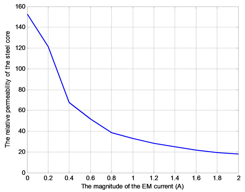
Figure 10. The estimated relative permeability values versus the EM currents.
for 30 minutes and the experiment was repeated for a new current. Figure 11 shows the result. It is noted when the current is low, the temperature increase is relatively slow and when the current is high, say above 1.0 A, the temperature increases drastically.The results indicate that the relative permeability change is not entirely attributed to the core temperature change. It is well known that the magnetic permeability of low-carbon steel materials quickly becomes saturated when the magnetic field is increased. Thus the magnetic saturation is used to explain why the relative permeability change is high when the current magnitude is small.
With the estimated relative permeability values, the model of Figure 6 was used to study how the EM current and the gap distance affect the stiffness of the EM spring. Figure 12 demonstrates the forces of the EM spring for four EM currents at D = 76.0 mm when the PM is placed at different locations. From these relationships, the corresponding stiffness values of the EM spring can be obtained, as shown in Figure 13. It can be observed that with an increase of the current, the EM stiffness becomes more negative.
3.3. The Passive HSLDS Isolator
When the mass-beam assembly is placed between the electromagnets that are not energized, a passive HSLDS isolator is obtained. To simulate the passive HSLDS isolator, a multiphysics functionality is required as it involves two physics, namely, structural mechanics and electromagnetism. Comsol software provides two ways to tackle a multiphysics problem: fully coupled and weakly coupled. In order to simplify the simulation, a “weakly coupled” way was employed in this study. This method solves for one type of physics at a time and then uses that solution as the initial value to solve for the other type of physics [13].

Figure 11. The core temperature vs the EM current.
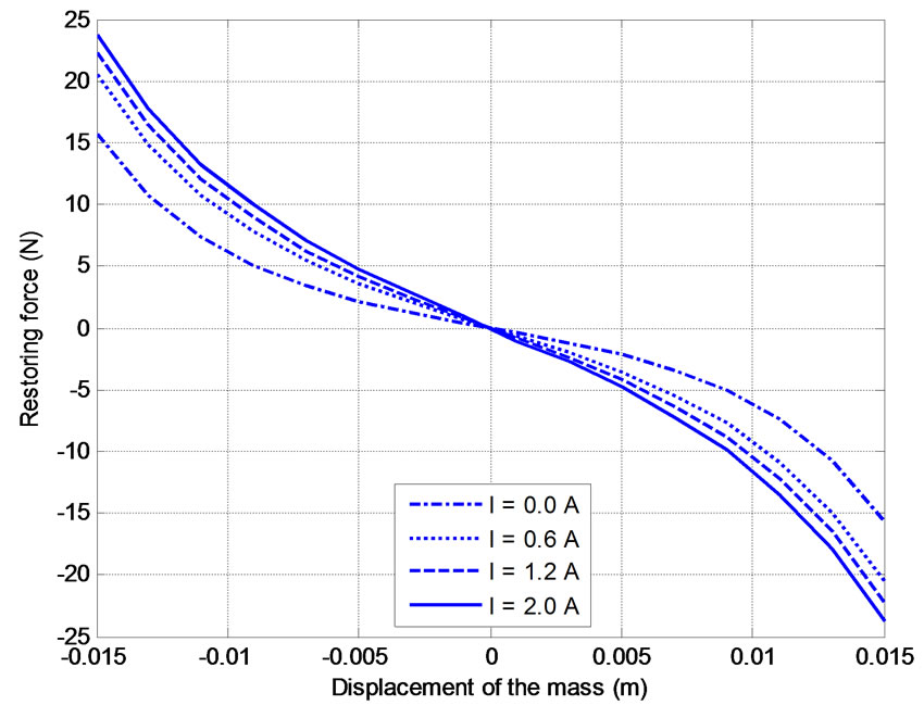
Figure 12. The net force acting on the PM for four EM currents at D = 76.0 mm.
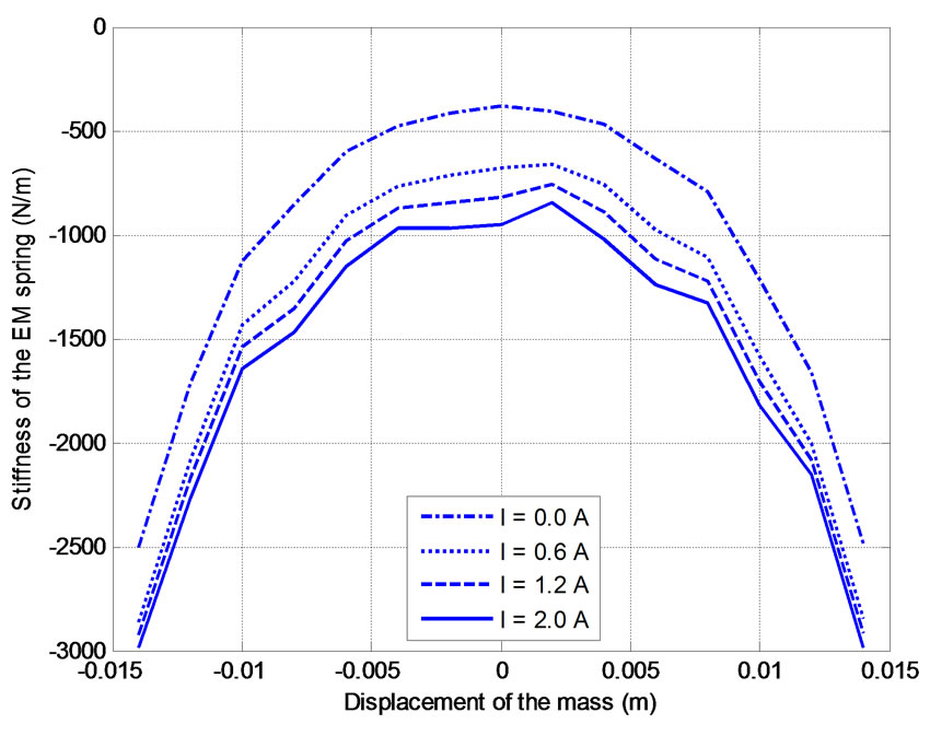
Figure 13. Stiffness of the EM spring for four EM currents at D = 76.0 mm.
As shown in Figure 14, the total restoring force of the passive isolator spring is given by:
 (4)
(4)
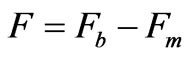
where Fb is the restoring force of the beam and Fm is the net magnetic force. Both Fb and Fm depend on the location of the mass. When the model shown in Figure 3 is run under the Structural Mechanics module, F = Fb. Therefore, by applying a force to the mass, the displacement of the mass can be found. Then the mass position in the model of Figure 6 is adjusted to this position and the model is run under the AC/DC module to find the corresponding force Fm. With Fb and Fm, the total restoring force F is obtained using Equation (4). This process was automated through a Comsol script. Figure 15 shows the total restoring forces versus the mass displacement for four gap distances. Figure 16 demonstrates the corre-

Figure 14. Forces acting on the mass.
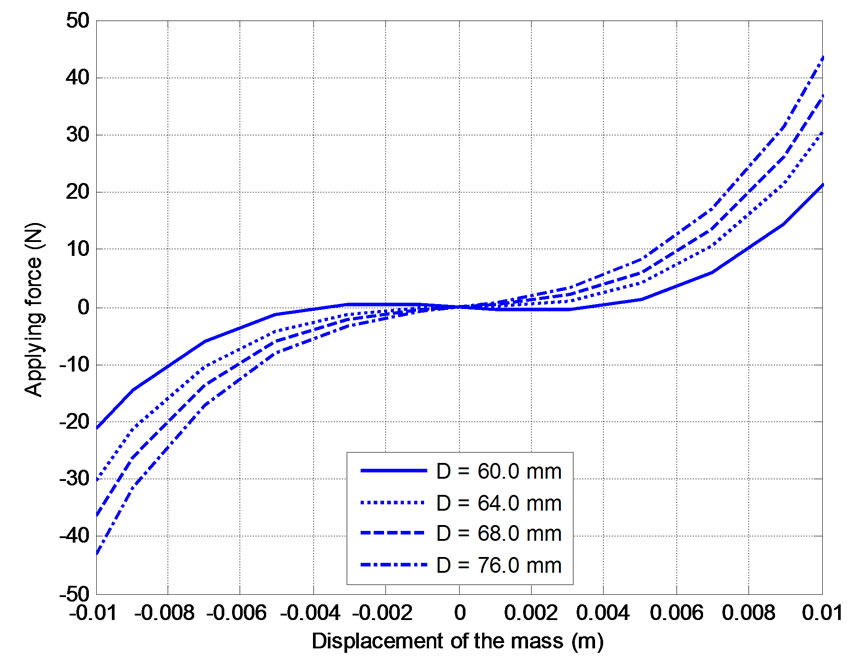
Figure 15. Total restoring forces versus the mass displacements for four different gap distances.
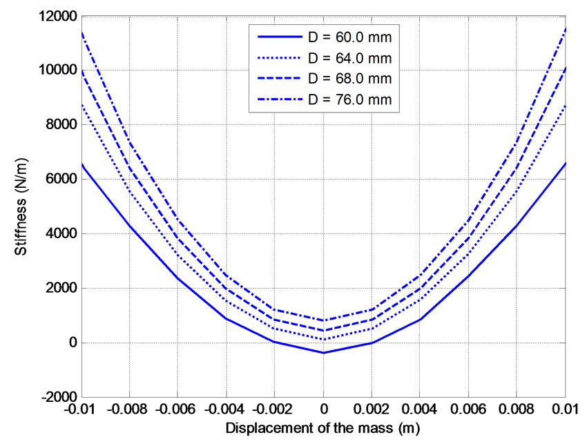
Figure 16. Dynamic stiffness values of the passive isolator for four different gap distances.
sponding stiffness curves. It can be observed that reducing the gap distance will lower the isolator stiffness. When the gap distance is too small, for example D = 60.0 mm, the isolator stiffness in the neighbourhood of the equilibrium position becomes negative, resulting in an unstable system.
3.4. The Tunable HSLDS Isolator
When the electromagnets are energized, the isolator’s stiffness becomes on-line tunable. The weakly coupled approach was again used to determine the total restoring forces of the isolator spring. Figure 17 shows the curves of the total restoring force versus the mass displacement for four different EM currents when the gap distance of the isolator is 76.0 mm. Figure 18 demonstrates the corresponding stiffness curves. It can be seen that increasing the EM current causes the isolator’s stiffness to decrease.
4. Displacement Transmissibility Ratio
The previous section has shown that the dynamic stiffness of the isolator can be reduced by either reducing the
Figure 17. Total restoring forces of the isolator spring for four EM currents at D = 76.0 mm.

Figure 18. Dynamic stiffness values of the isolator spring for four EM currents at D = 76.0 mm.
gap distance or by increasing the EM current. In this Section, the performance of the isolator is investigated by evaluating the displacement transmissibility ratio (T.R.). First the T.R. is defined. When a vibration isolator is subjected to a sinusoidal base excitation given by
 (5)
(5)
where Y and ωb are the amplitude and frequency of the base motion, respectively. The steady-state response of the isolated mass is given by
 (6)
(6)
where X and θ are the amplitude and phase of the steadystate response of the isolated mass, respectively. The displacement transmissibility ratio (T.R.) is defined as
 (7)
(7)
when T.R. < 1, the vibration isolation occurs.
Because the isolator stiffness is nonlinear, a closedform solution for its T.R. does not exist. In this study, a numerical solution was conducted using Comsol multiphysics package. Several attempts were made. One attempt was to use the weakly coupled method. It failed due to an enormous computational burden and convergence problem. In another attempt, the magnetic spring was treated as a lumped-parameter element whose restoring force equations were determined from the results presented in Section 3.2. This lumped-parameter spring was added to the model shown in Figure 3. The timedependent solver provided in the Structural module was used to find the response of the mass to a given base motion. The simulation worked when the frequency of the base motion was away from the natural frequency of the system. However, when the frequency of the base motion was close to the natural frequency of the base motion, the simulation failed to converge. To avoid the aforementioned difficulties, the isolator was simplified as a lumped-parameter system and its equation of motion is given by:
 (8)
(8)
where m is the mass, c is the damping coefficient, z = x − y is the relative displacement of the mass, and f(z) is the restoring force of the isolator spring. For the passive isolator, the restoring force is obtained by adding the restoring force of the beam (solid line in Figure 4) and the restoring force of the magnetic spring (Figure 7). For the semi-active isolator, the restoring force is obtained by adding the restoring force of the beam and the restoring force of the electromagnetic spring (Figure 12). By assigning y = Ysin(ωbt) as the base motion and using z = x − y, Equation (8) is rewritten as
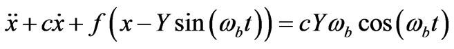 (9)
(9)
The above equation was imported in the global equation dialog box in the Structural Mechanics module. The time-dependent solver was employed to solve the equation.
The damping coefficient was estimated by the following procedure. First, a free response experiment was conducted on the passive isolator. In the experiment, the mass was displaced by 2.26 mm and released. The induced free response was measured. Using the measured free response, the damping coefficient was estimated to be c = 0.13 Ns/m. Then a Comsol simulation was conducted with c = 0.13 Ns/m as a trial damping coefficient. The simulated response was compared with the measured one. The simulation was repeated by varying the trial damping coefficient values. The damping coefficient that resulted in the best agreement between the simulated response and simulated one was chosen to be the value used in the following simulations. Figure 19 compares the measured response and simulated one with the damping coefficient obtained using the above procedure.
The amplitude of the sinusoidal base motion was taken as 1.0 mm and the initial conditions were zero. It was observed that the response became almost steady state after 24.0 seconds. A Comsol script was used to compute the RMS value of the response in the duration of 24.0 second and 30.0 second. The transmissibility ratio was computed using the ratio of the RMS value of the mass displacement over that of the base motion. By varying the exciting frequency from 1.0 Hz to 25.0 Hz in a step size of 0.5 Hz, the relationship between the transmissibility ratio and the base exciting frequency was obtained.
Figure 20 compares the T.R. values of the passive isolator for four different gap distances: D = ∞ mm or
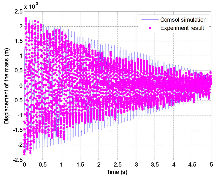
Figure 19. The measured response and simulated response of the mass subject to an initial displacement 2.26 mm.
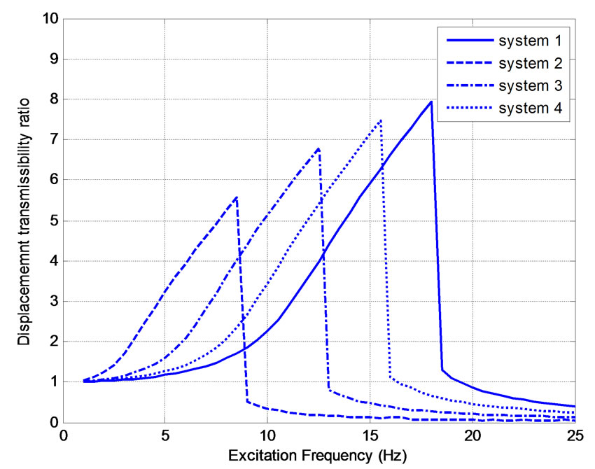
Figure 20. The measured response and simulated response of the mass subject to an initial displacement 2.26 mm.
with the mechanical spring only (System 1), D = 64.0 mm (System 2), D = 68.0 mm (System 3), and D = 76 mm (System 4). Several observations can be drawn. With the mechanical spring only or System 1, the transmissibility ratio increases with an increase of the exciting frequency up to about 18 Hz. After that, the transmissibility ratio drops drastically. A further increase of the exciting frequency makes the value of the transmissibility ratio less than one. A sudden jump in the amplitude of the steady-state response is a typical phenomenon in systems with a hardening or softening stiffness [7,17]. In this paper, the lowest exciting frequency that causes such a jump phenomenon is referred to as the jump frequency. With the influence of the PM spring (Systems 2, 3, 4), the pattern of the transmissibility ratio curve remains similar but the jump frequency shifts to the left when the gap distance decreases. This indicates that the introduction of the PM spring widens the vibration isolation region. It is also noted that the PM spring causes an increase of the transmissibility ratio in the low frequency region.
The same process was employed to compute the transmissibility ratios for the semi-active isolator with a gap distance of D = 76 mm. Figure 21 shows the results of four cases. Note that the restoring forces of the spring of the four cases are given in Figure 17. From Figure 21, it can be seen that with an increase of the EM current, the pattern of the transmissibility ratio curve remains similar but the jump frequency shifts to the left and the vibration isolation region is widened. It is also noted that with an increase of the EM current, the transmissibility ratio in the low frequency region increases.
5. Conclusions
The characterization study for a novel vibration isolator
Figure 21. Transmissibility ratios of the semi-active isolator with D = 76.0 mm: I = 0.0 A (solid line); I = 0.6 A (dashed line); I = 1.2 A (dash-dotted line); I = 2.0 A (dotted line).
has been conducted using Comsol Multiphysics package. The stiffness behaviors of both the mechanical spring and magnetic spring have been determined. The study has shown that the mechanical spring possesses a positive nonlinear stiffness while the magnetic spring possesses a negative nonlinear stiffness. The simulation has shown that the stiffness of the magnetic spring can be varied by either changing the gap distance or the current. Using the weakly-coupled multiphysics approach, the combined stiffness of the passive isolator has been investigated. It has been found that the HSLDS property of the passive isolator can be tuned by varying the gap distance of the EMs. Using the weakly-coupled multiphysics approach, the combined stiffness of the semi-active isolator has been investigated. It has been found that the HSLDS property of the semi-active isolator can be varied by varying the EM current. A lumped-parameter model has been used to simulate the dynamic responses of the passive isolator and semi-active isolator to a base excitation. The obtained relationships between the transmission ratio and the exciting frequency have verified that the isolation region of the isolator can be effectively widened by either reducing the gap distance or increasing the current of the electromagnets. This study has demonstrated that a multi-physics finite element package can be used to tackle a nonlinear system that involves two different physics. The study has also shown that an experimental calibration or validation is critical in order to obtain a reliable computer simulation using a finite element based package.
REFERENCES
- D. J. Mead, “Passive Vibration Control,” John Wiley & Sons Ltd., Chichester, 1999.
- G. Coppola and K. Liu, “Control of a Unique Active Vibration Isolator with a Phase Compensation Technique and Automatic on/off Switching,” Journal of Sound and Vibration, Vol. 329, No. 25, 2010, pp. 5233-5248. doi:10.1016/j.jsv.2010.06.025
- G. Coppola, “On the Control Methodologies of a Novel Active Vibration Isolator,” M.Sc. Thesis, Lakehead University, Thunder Bay, 2010.
- G. Falsone and G. Ferro, “Best Performing Parameters of Linear and Non-Linear Seismic Base-Isolator Systems Obtained by the Power Flow Analysis,” Computers and Structures, Vol. 84, No. 31-32, 2006, pp. 2291-2305. doi:10.1016/j.compstruc.2006.08.068
- N. Zhou, K. Liu, X. Liu and B. Chen, “Adaptive Fuzzy Control of an Active Vibration Isolator,” Proceedings of the 8th International Conference on Advances in Neural Networks, Guilin, 29 May-1 June 2011, pp. 552-562.
- A. Carrella, M. J. Brennan, T. P. Waters and K. Shin, “On the Design of a High-Static-Low-Dynamic Stiffness Isolator Using Linear Mechanical Springs and Magnets,” Journal of Sound and Vibration, Vol. 315, No. 3, 2008, pp. 712-720.doi:10.1016/j.jsv.2008.01.046
- A. Carrella, “Passive Vibration Isolators with High-StaticLow-Dynamic-Stiffness,” Ph.D. Thesis, University of Southampton, Southampton, 2008.
- Y. Liu, H. Matsuhisa and H. Utsuno, “Semi-Active Vibration System with Variable Stiffness and Damping Control,” Journal of Sound and Vibration, Vol. 313, No. 1-2, 2008, pp. 16-28.doi:10.1016/j.jsv.2007.11.045
- Y. Liu, T. P. Waters and M. J. Brennan, “A Comparison of Semi-Active Damping Control Strategies for Vibration of Harmonic Disturbances,” Journal of Sound and Vibration, Vol. 280, No. 1-2, 2005, pp. 21-39. doi:10.1016/j.jsv.2003.11.048
- M. M. ElMadany and A. El-Tamimi, “On a Subclass of Nonlinear Passive and Semi-Active Damping for Vibration Isolation,” Computers and Structures, Vol. 36, No. 5, 1990, pp. 921-931.doi:10.1016/0045-7949(90)90163-V
- N. Zhou and K. Liu, “A Tunable High-Static-Low-Dynamic Stiffness Vibration Isolator,” Journal of Sound and Vibration, Vol. 329, No. 9, 2010, pp. 1254-1237. doi:10.1016/j.jsv.2009.11.001
- N. Zhou, “A Tunable High-Static-Low-Dynamic-Stiffness Isolator and Fuzzy-Neural Network Based Active Control Isolator,” M.Sc. Thesis, Lakehead University, Thunder Bay, 2009.
- AC/DC Module Model Library, “Comsol Multiphysics Manual,” 2006.
- I. E. Harik and X. J. Zheng, “FE-FD Model for Magneto-Elastic Buckling of Ferromagnetic Plates,” Computers and Structures, Vol. 61, No. 6, 1996, pp. 1115-1123. doi:10.1016/0045-7949(96)00118-6
- M. Modarres, A. Vahedi and M. Ghazanchaei, “Study on Axial Flux Hysteresis Motors Considering Airgap Variation,” Journal of Electromagnetic Analysis and Applications, Vol. 2, No. 4, 2010, pp. 252-257. doi:10.4236/jemaa.2010.24031
- T. Zedler, A. Nikanorov and B. Nacke, “Investigation of Relative Magnetic Permeability as Input Data for Numerical Simulation of Induction Surface Hardening,” Proceedings of the International Scientific Colloquium, Modelling for Electromagnetic Processing, Hannover, 26-29 October 2008.
- M. J. Brennan, I. Kovacic, A. Carrella and T. P. Waters, “On the Jump-Up and Jump-Down Frequencies of the Duffing Oscillator,” Journal of Sound and Vibration, Vol. 318, No. 4-5, 2008, pp. 1250-1261. doi:10.1016/j.jsv.2008.04.032