ABSTRACT

The main properties (attenuation along the surface, attenuation in depth, additional radiation in depth, dispersion in propagation space) of Bleustein-Gulyaev surface acoustic waves (SAWs) in electroelasticity are determined in terms of a perturbation due to viscosity. This paves the way for a study of the perturbed motion of associated quasi-particles in the presence of low losses.

1. Introduction

In two previous papers [1,2] we have shown how quasiparticles in inertial motion could be associated canonically with surface acoustic waves (SAWs) of the Rayleigh and Bleustein-Gulyaev types, in the absence of dissipation. A natural extension of this kind of approach is the consideration of the possible non-inertial motion of quasi-particles that would be associated with these surface waves in presence of dissipation. The latter can be of purely mechanical origin (viscosity, plasticity, damage) in the Rayleigh case and of mixed mechanical and electrical origins—the last property being related to phenomena such as polarization relaxation, hysteresis, etc.— for Bleustein-Gulyaev waves. The Rayleigh case inevitably involves two elastic displacements and this greatly complicates any analytic treatment. Accordingly, we consider here the case of Bleustein-Gulyaev waves which, although coupling small strains with an electric potential, remains with a single elastic (SH = shearhorizontal) displacement [3,4]. Furthermore, while electric dissipation would change the nature of the dynamical problem, after a general introduction we envisage only the influence of mechanical dissipation in the form of viscosity. Very few works have considered the dissipative propagation of Bleustein-Gulyaev waves. The work of Romeo [5] is an exception. The dissipative Rayleigh case was more often considered (cf. Caloi [6], Scholte [7], Tsai and Kolsky [8], Curie et al. [9], Curie and O’Leary [10], Romeo [11], Lai and Rix [12], Acharya and Mondal [13], Addy and Chakraborty [14], Carcione [15]). But none of these could envisage the association of quasi-particles with SAWs so that the present work appears to be the first of its kind. This association will be dealt with in an extension of this work, once we have established a consistent direct “analytic-approximate” solution in this first part, the quasi-particle approach having most of the time a different purpose, that of treating the main elements of perturbations of the known exact linear solution by various factors (dissipation, nonlinearity, interactions with “obstacles”). But we do need this solution and exhibiting it is the main purpose of this paper.

2. Reminder of General Piezoelectricity in the Presence of Dissipative Effects

2.1. Balance Laws and Constitutive Equations

We use indifferently the intrinsic (with no indices) notation or the indexed Cartesian tensor notation. Here the symbol or a superimposed dot denotes the partial time derivative. The symbol stands for the gradient (e.g., in components,); div means the divergence of second order tensors (e.g.,). provides a system of rectangular coordinates and the time parametrization by the Newtonian time t. Symbol u will denote the elastic displacement. Accordingly, in any regular material point of the considered piezoelectric body the local balance of linear momentum and Gauss equation read:

.(2.1)

Here is the linear momentum, σ is Cauchy’s (symmetric) stress tensor, D is the electric displacement, is the constant matter density, and u is the elastic displacement. Any body force is discarded. Only small strains and weak electromagnetic fields are considered. The theory is linear so that both electromagnetic ponderomotive force and couple that are basically quadratic in the fields are discarded (for these see Maugin, 1988 [16]). The electric framework is that of quasi-electrostatics (no electromagnetic inertia, Maxwell’s equations reduced to (2.1 2) and, so that the electric field vector E derives from the potential i.e., , but all fields still depend on time). The electric displacement vector D is such that

(2.2)

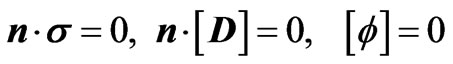
where is the vacuum electric permeability, and P is the electric polarization vector per unit volume. LorentzHeaviside units are used (no factor 4π). Natural boundary conditions associated with Equation (2.1) read

(2.3a)

These hold for a mechanically free surface, and a connection to an external electric field in the vacuum outside the body, the symbolism indicating the finite jump of the enclosed quantity at the bounding surface, i.e., , where denotes the uniform limit of the function A in approaching the limit surface from the positive and negative sides of the surface, respectively, and n is the unit normal to the boundary oriented from the minus to the plus side. Whenever this surface is electroded fixing the electric potential on it, say (zero potential), then (2.3a) are replaced by

,(2.3b)

where w is an imposed surface density of electric charges. This is the case mostly considered in the present work. Type (2.3a) is briefly considered in Section 4 below.

In the presence of dissipation of the viscous and electric-relaxation type the constitutive equations for σ and D are given in Cartesian tensor components by

,(2.4)

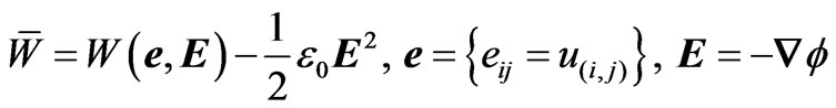
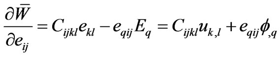
The nondissipative contributions here derivable from the volume energy are the standard ones given by the theory of linear piezoelectricity (cf.Maugin, 1988 [16]; Chapter 4):

,(2.5)

,(2.6.1)

, (2.6.2)

where (quadratic energy)

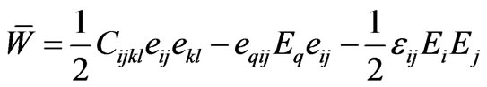,(2.7)

with the following symmetries:

,(2.8)

for the tensorial coefficients of elasticity, piezoelectricity and dielectricity, respectively. The field e of components stands for the small strain tensor, and parentheses around a set of indices indicate the operation of symmetrization.

Simple examples of dissipative contributions in the context of Bleustein-Gulyaev waves are given by (cf. Maugin et al, 1992 [17]); a superimposed dot is the same as the partial time derivative)

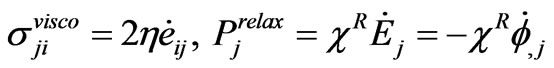,(2.9)

with positive viscosity and relaxation constant. A symmetry class (no center of symmetry) allowing for the existence of piezoelectricity must be selected for (2.8). Simple isotropy has been considered for the dissipative effects, bearing no restriction for the application in this paper.

For the case of Bleustein-Gulyaev surface acoustic waves (SAWs) with elastic displacement polarized orthogonally to the sagittal plane spanned by the propagation direction and the in-depth coordinate, the only surviving components of (2.3) are given by (compare the nondissipatif case in Maugin and Rousseau, 2010 [2])

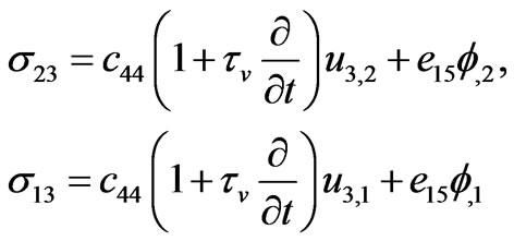,(2.10)

. (2.11)

with

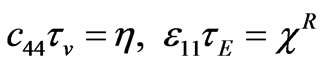.(2.12)

Here, and are the only intervening elasticity, piezoelectric and dielectric constants (in the socalled Voigt’s notation commonly used in piezoelectricity).

Of course, the corresponding wave problem becomes dispersive since the polynomials of differentiation are no longer homogeneous.

2.2. Energy Equation

If we multiply (2.1.1) by and sum over indices, we obtain

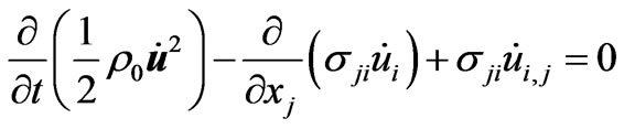,(2.13)

or, on account of (2.4),

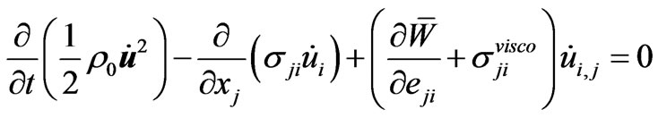.(2.14)

But (2.1.2) yields

. (2.15)

Subtracting the (vanishing) right-hand side of (2.15) from (2.14) yields the (non)-conservation of energy in the form

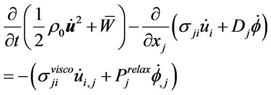. (2.16)

Remark: Equation (2.16) has a remarkable symmetric structure for mechanical and electric effects. Quite often, however, the Poynting vector for quasi-electrostatic fields is written as

,(2.17)

[cf. Maugin, 1988, Equation (4.6.14), p.238 [16]; or Eringen and Maugin, 1990, Equation (7.3.15) [18], p. 246]. This can be accommodated by Equation (2.16) by a re-definition of the energy W. For instance, we can rewrite (2.16) as

(2.18)

With

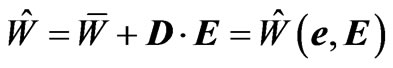. (2.19)

Obviously, (2.18) is less convenient than (2.16) for our purpose. While the SAW problem is based on an exploitation of Equation (2.1) and accompanying boundary conditions, that of the formulation of the mechanics of associated quasi-particles (subsequent work) is based on an exploitation of Equation (2.16) and of an analogous spatial co-vectorial equation known as the conservation (or non-conservation) of wave momentum. (general concept in Maugin, 2011 [19]; Chapter 12), once the SAW solution is known, just like in a post-processing procedure. This completes the thermo-electromechanical modeling per se.

3. Surface BG Wave Solution in the Presence of Low Viscous Losses Only

The dissipative case will be treated along the same line as the known BG solution but with account of a perturbation by low viscous processes only.

3.1. Reminder of the Pure BG SAW Solution

In this case, after introduction of an effective scalar electric potential, the surviving Equation (2.1) for the fields are

.(3.1)

with

,(3.2)

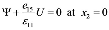
where K is the so-called electromechanical coupling factor. The boundary conditions (2.3b1,3) at the mechanically free, but electrically grounded surface, yield

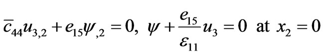(3.4)

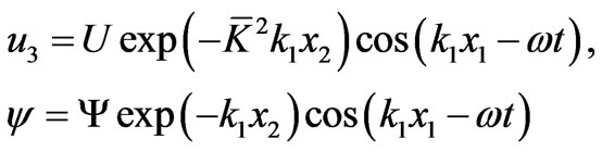
For the half-space, the SAW solution generally reads

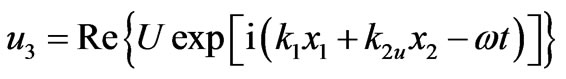(3.5)

.(3.6)

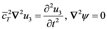
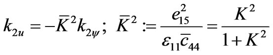
From (3.1.1) and (3.1.2) there follows that

(3.7)

and (3.1.2) is not a propagation equation

.(3.8)

That is,

.(3.9)

The boundary conditions (3.4) yield a nontrivial solution for

.(3.10)

The first of these has to be substituted in (3.7.1) on account of (3.10)₂. This yields

from which there follows the “dispersion relation” of Bleustein-Gulyaev surface waves for the present electric boundary condition:

.(3.11)

Noting that, the real BG SAW for can be written as the solution

,(3.12)

with

.(3.13)

For a vanishing electromechanical coupling coefficient, the surface wave degenerates into a face shear wave (cf. Equation (3.12.1) for). Consistently with (3.11), we note and the wave parameters (velocity, wave number and wavelength) of this solution. Those corresponding to a dissipatively perturbed solution will be denoted with an additional subscript d, e.g., , etc.

3.2. BG SAW Solution Including Low Viscous Losses

For the sake of simplicity we discard dielectric relaxation. Constitutive Equations (2.10) and (2.11) reduce to

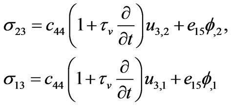, (3.14)

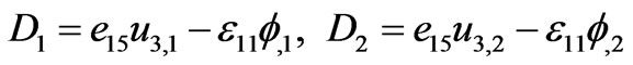, (3.15)

with.

We follow the same strategy as for the nondissipative case recalled in the preceding paragraph. The ansatz SAW solution is like in Equations (3.5)-(3.6) but with all k’s now possibly complex. The dimensionless parameter defined by

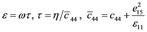,(3.16)

that compares the viscous relaxation time to the time scale of the wave motion, is considered as an infinitesimally small quantity of the first order, so that in the sequel. Relation (3.1.3) is still valid, so that together with (3.1) and (3.2) Equations (2.1) reduce to the following system:

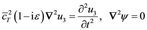,(3.17)

for, with conditions (2.3.b1,3) at, i.e.,

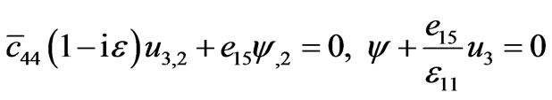.(3.18)

Equations (3.7) are replaced by the following ones:

(3.19)

and

.(3.20)

Whence,

.(3.21)

Finally, (3.11.1) is replaced by the following—still exact—complex (true) dispersion relation

,(3.22)

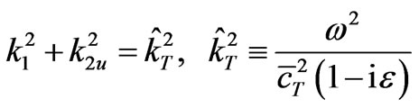
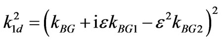
with defined in (3.11.2). Let the complex wave-number solution of (3.22). We have thus

(3.23)

where.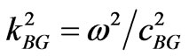

Now we look for approximations of in terms of. We write for the left-hand side of (3.23)

,(3.24)

or at order,

.(3.25)

At the same order of approximation the right-hand side of (3.23) yields

.(3.26)

Identifying the like powers of from (3.25) and (3.26), we can draw the following conclusions.

•     At order zero in we obviously have the solution provided by (3.11);

•     At order one in, we have (K being small by itself) :

;(3.27)

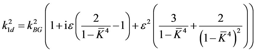
•     At order two in, we obtain:

,(3.28)

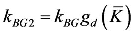
with

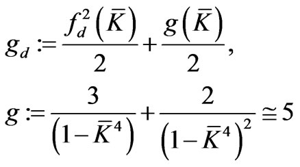. (3.29)

This solution is completed by applying the same approximation to the relation given by (3.9).

That is, we can write

. (3.30)

This manipulation yields

. (3.31)

We also show that

.(3.32)

The SAW solution finally reads

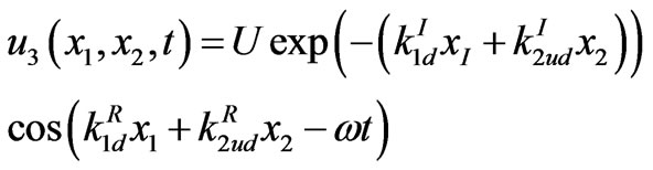,(3.33)

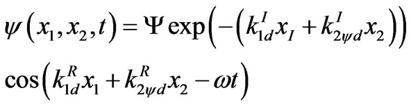,(3.34)

where superscripts I and R denote imaginary and real parts, respectively. Summing up, we have up to order:

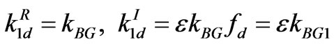,(3.35)

(3.36)

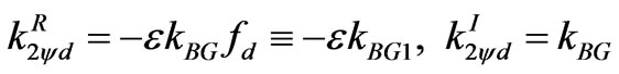. (3.37)

Globally, we see that at order:

•     yields attenuation in the propagation direction. This is of order of.

•     yields the expected exponential attenuation in depth for a surface wave.

•     yields a superimposed oscillation in depth (due to the viscous behavior).

We also remark that at order, describes dispersion in the propagation direction. This dispersion that varies like, results from the viscous behavior.

4. Other Case of Electric Boundary Condition

For the sake of completeness we also briefly consider the other standard case (2.3a) of boundary conditions at. Thus,

, (4.1)

i.e., the matching with a vacuum half-space above the limiting plane. Since there is no matter in the region and is the vacuum dielectric constant, we shall complement the solution (3.5)-(3.6) by considering

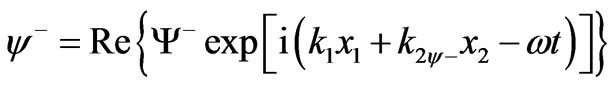(4.2)

with

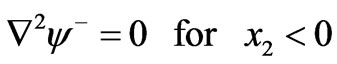. (4.3)

On account of pure viscous dissipative processes and applying the conditions (4.1.1,3) we find that

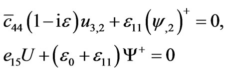.(4.4)

We obtain thus (3.19) and

,(4.5)

.(4.6)

Thus, the coupling coefficient replaces in the solution given in Section 3, while the complex dispersion relation is obtained in a form similar to (3.22) or (3.23). But remember that all k’s are a priori complex and in addition to expression of the form (3.33) and (3.34) for and with amplitude, we shall have for a real electric potential solution

, (4.7)

with an oscillation behavior combined with an exponential decrease in the negative direction. We do not pursue the detail of this solution, noting simply that the introduction of associated quasi-particles would require the consideration of an integration over the whole axis (compare the nondissipative case in Section 6 of Maugin and Rousseau, 2010 [2]).

5. Conclusive Remarks

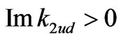
The above given results—we believe reported for the first time in a clear cut manner, show how complex can become the behavior of the relevant surface waves in the presence of dissipation. The somewhat annoying property is the one exhibited by the relation, indicating that propagation is no longer purely along, hence a radiation along the axis, and a propagation direction at an—although small—angle to the direction in the sagittal plane. Dispersion is a less dramatic effect as being of order. These are interesting and they would themselves lend to experimental investigations. But our own purpose was to obtain an analytical solution which, although approximate, is needed to exploit the conservation laws of energy and wave momentum (of which the general features are studied in Ref. [19]) in order to define without ambiguity the notion of associated quasi-particle (compare References 1 and 2 in the absence of losses). This will be achieved in a further work. Note that this notion of quasi-particle—in the expected duality between wave and particle that is very original for surface waves—will be useful in studying problems involving encounter with an obstacle placed on the path of the wave, e.g., experimentally, in nondestructive evaluation techniques.

REFERENCES

- M. Rousseau and G. A. Maugin, “Rayleigh SAW and Its Canonically Associated Quasi-Particle,” Proceedings of the Royal Society of London, Vol. A 467, 2011, pp. 495- 507. doi:10.1098/rspa.2010.0229
- G. A. Maugin and M. Rousseau, “Bleustein-Gulyaev SAW and Its Associated Quasi-Article,” International Journal of Engineering Science, Vol. 48, No. 11, November 2010, pp. 1462-1469. doi:10.1016/j.ijengsci.2010.04.016
- J. L. Bleustein, “A New Surface Wave in Piezoelectric Materials,” Applied Physics Letters, Vol. 13, No. 12, 1968, pp. 412-414. doi:10.1063/1.1652495
- Y. V. Gulyaev, “Electroacoustic Surface Waves in Solids,” ZhETF Pis ma Redaktsiiu, Vol. 9, 1969, pp. 35- 38.
- M. Romeo, “A Solution for Transient Surface Waves of the B-G Type in a Dissipative Piezoelectric Crystal,” Zeitschrift für Angewandte Mathematik und Physik (ZAMP), Vol. 52, No. 5, 2001, pp. 730-748.
- P. Caloi, “Comportement des ondes de Rayleigh dans un milieu firmo-élastique indéfini,” Publ. Bureau Central Seismol. Internat., Sér. A. Travaux scientifiques, Vol. 17, 1950, pp. 89-108.
- J. G. Scholte, “On Rayleigh Waves in Visco-Elastic Media,” Physica (Utrecht), Vol. 13, No. 4-5, May 1947, pp. 245-250. doi:10.1016/0031-8914(47)90083-9
- Y. M. Tsai and H. Kolsky, “Surface Wave Propagation for Linear Viscoelastic Solids,” Journal of the Mechanics and Physics of Solids, Vol. 16, No. 2, March 1968, pp. 99-109. doi:10.1016/0022-5096(68)90008-2
- P. K. Curie, M. A. Hayes and P. M. O’Leary, “Viscoelastic Rayleigh Waves,” Quarterly of Applied Mathematics, Vol. 35, 1977, pp. 35-53.
- P. K. Curie and P. M. O’Leary, “Viscoelatic Rayleigh Waves II,” Quarterly of Applied Mathematics, Vol. 35, 1978, pp. 445-454.
- M. Romeo, “Rayleigh Waves on a Viscoelastic Solid Half-Space,” The Journal of the Acoustical Society of America, Vol. 110, No. 1, 2001, pp. 59-67. doi:10.1121/1.1378347
- C. G. Lai and G. L. Rix, “Solution of the Rayleigh Eigenproblem in Viscoelastic Media,” Bulletin of the Seismological Society of America, Vol. 92, No. 6, 2002, pp. 2297-2309. doi:10.1785/0120010165
- D. P. Acharya and A. Mondal, “Propagation of Rayleigh Waves with Small Wavelength Innonlocal Visco-Elastic Media,” Sadhana, Vol. 27, No. 6, 2002, pp. 605-612.
- S. K. Addy and N. R. Chakraborty, “Rayleigh Waves in a Viscoelastic Half-Space under Initial Hydrostatic Stress in Presence of the Temperature Field,” International Journal of Mathematics Sciences, Vol. 24, 2005, pp. 3883-3894. doi:10.1155/IJMMS.2005.3883
- J. M. Carcione, “Rayleigh Waves in Isotropic Viscoelastic Media,” Geophysical Journal International, Vol. 108, No. 2, 2007, pp. 453-464. doi:10.1111/j.1365-246X.1992.tb04628.x
- G. A. Maugin, “Continuum Mechanics of Electromagnetic Solids,” North-Holland, Amsterdam, 1988.
- G. A. Maugin, J. Pouget, R. Drouot and B. Collet, “Nonlinear Electromechanical Couplings,” John Wiley & Sons, New York, 1992.
- A. C. Eringen and G. A. Maugin, “Electrodynamics of Continua,” Springer, New York, 1990.
- G. A. Maugin, “Configurational Forces: Thermomechanics, Physics, Mathematics, and Numerics,” CRC/Taylor and Francis, Boca Raton, Florida, 2011.