Journal of Electromagnetic Analysis and Applications
Vol. 3 No. 6 (2011) , Article ID: 5351 , 8 pages DOI:10.4236/jemaa.2011.36032
Non Linear Magnetic Hysteresis Modelling by Finite Volume Method for Jiles-Atherton Model Optimizing by a Genetic Algorithm
![]()
1DIMMER, Laboratory of Microwaves Devices and Materials for Renewable Energy, Department of Sciences Technology, University of Djelfa, Djelfa, Algeria; 2LESM, Laboratory of Energy Systems Modeling, University of Biskra, Biskra, Algeria; 3Professeur des Universités, LIME-IUT de Brest, Université de Bretagne Occidentale, Brest, France.
Email: azzaoui_seddik@yahoo.fr, ksrairi@yahoo.fr, m.benbouzid@ieee.org
Received February 25th, 2011; revised April 8th, 2011; accepted May 10th, 2011.
Keywords: Magnetic Hysteresis, Jiles-Atherton Model, Genetic Algorithm Optimization, Parameters Identification, Finite Volume Method (FVM)
ABSTRACT
This paper describes a generalization methodology for nonlinear magnetic field calculation applied on two-dimensional (2-D) finite Volume geometry by incorporating a Jiles-Atherton scalar hysteresis model. The scheme is based upon the definition of modified governing equation derived from Maxwell’s equations considered the magnetization M. This paper shows how to extract optimal parameters for the Jiles-Atherton model of hysteresis by a real coded genetic algorithm approach. The parameters identification is performed by minimizing the mean squared error between experimenttal and simulated magnetic field curves. The calculated results are validated by experiences performed in an SST’s frame.
1. Introduction
Numerical electromagnetic is the theory and practice of solving electromagnetic field problems on digital computers. It reflects the general trend in science and engineering to formulate the laws of nature as computer algorithms and to simulate physical processes on digital computers. While theory and experiment remain the two traditional pillars of science and engineering, numerical modeling and simulation represent a third pillar that supports, complements, and sometimes replaces them. For this reason, the objective of this work is therefore to study for modeling, magnetic hysteresis, to integrate it into a computer code field. Different hysteresis models are available for incorporation into the finite volume framework. Although the Preisach model appears to be the hysteresis model of choice, the J-A model is attracttive because of its simplicity and ease of implementtation. The attributes of the J-A hysteresis model includeing level of accuracy for several practical materials, ease of implementation into the FVM (Finite Volume Method), and computational efficiencies make it a viable choice for implementation into a 2-D finite Volume model [1], [2]. This study will choose the model best suited from the standpoint accuracy, processing speed and ease of implementation. The working hypotheses are restricted to the case of static regime and the equation that we solve axi-symmetrical in two dimensions 2-D, is the non-linear magnetodynamic. Thus, the finite element method has proved it self as an effective tool in solving differential equations, it allows another to take into account complex geometries and non-linearity’s possible, only its implementation is against a fairly complicated. So we choose in our study for the method of finite Volume, which is less difficult to achieve and simple design.
2. Finite Volume Formulations Including Magnetic Hysteresis
2.1. Basic Field Axi-Symmetrical Equations
The derivation of the finite Volume equations begins with Maxwell’s field equations
 (1)
(1)
 (2)
(2)
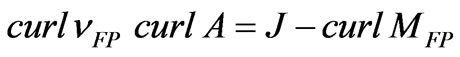
The Maxwell field equations are extended to allow treatment of hysteresis by including the constitutive equation for magnetic material. The general equation for a ferromagnetic material can be expressed as
 (3)
(3)
where  the nonlinear magnetization is function, and
  is the permeability in free space [1]. The flux density
  can be expressed as the circulation of a potential vector,
  , where
  is the magnetic vector potential naturally satisfying Maxwell’s equation
  since the divergence of the curl is zero. The most obvious way is to directly use μ0 (or
 ) and
) and  in the field equation by applying the vector form of (3) Ampere’s law. The field equation is then given by
 (4)
(4)
where ,
,  and
and  are, respectively, the magnetic vector potential, the current density, and the magnetization vectors at time
 , Δt is the time step.
When considering  as negligible in the azimuth direction (axis-symmetrical Formulation), (4) is written using the tow-dimensional (2-D) magnetic vector potential
  as unknown in cylindrical coordinates as
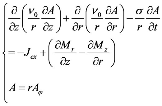 (5)
(5)
2.2. Jiles-Atherton Model of Hysteresis
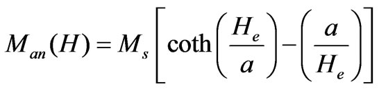
The original J-A model presented in [3] gives the magnetization M versus the external magnetic field H. This model is based on the magnetic material response without hysteresis losses. This is the anhysteretic behavior which Man (H) curve can be described with a modified Langevin equation
 (6)
(6)
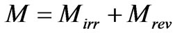
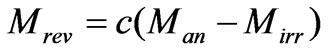
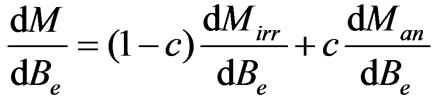
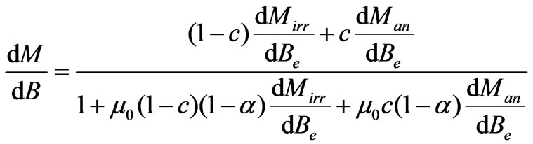
where He =H + αM is the effective field experienced by the domains, H is the external applied field and α is the mean field parameter representing inter-domain coupling. The constant a is an increasing function of the temperature. The magnetization M is decomposed into its reversible component Mrev and its irreversible component Mirr.
 (7)
(7)
The relationship between these two components and the anhysteretic magnetization Man is obtained from physical considerations of the magnetization process and is given by
 (8)
(8)
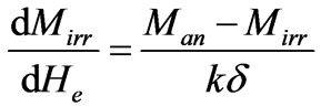
With
 (9)
(9)
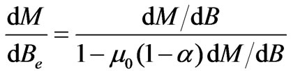
where a, α, c, k and the saturation magnetization Ms are parameters which are determined from measured hysteresis characteristics [4], δ is a directional parameter and takes the value +1 for dH/dt > 0 and –1 for dH/dt < 0. Using this method, the magnetization M is commonly obtained from the magnetic field H. With the proposed inverse Jiles-Atherton model, M will be calculated from the magnetic induction B, integrating a differential equation in terms of dM/dB. To obtain such a relationship, we will start substituting (8) in (7) and differentiating the resulting term with respect to the effective flux density Be = µ0He.
 (10)
(10)
 (11)
(11)
One can write this term as
 (12)
(12)
Deriving (6) with respect to He
 (13)
(13)
And, with deriving (9) results in
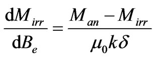 (14)
(14)
in which δ = + 1 for dB/dt > 0 and  for dB/dt < 0. The term Mirr in (14) is obtained applying (8) in (7)
 (15)
(15)
Finally, written (11) using (12) and (13), and isolating dM/dB gives the main equation of the proposed inverse Jiles-Atherton model
 (16)
(16)
The numerical solution of (5) including hysteresis cannot be done with the same method as the one used with univocal functions (Newton-Raphson scheme for example). We have chosen the fixed-point method already presented in [1]. The hysteretic constitutive relationship is then rewritten under the form
 (17)
(17)
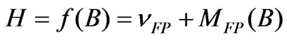
The reluctivity νFP is a constant and must respect some conditions to achieve convergence [2]. The studied hysteretic models assume B and H collinear; consequently the magnetization MFP has the same direction as νFP B. Its magnitude is obtained by calculating MPF= f(B) – νFP B. Finally, the partial differential equation (5) becomes
 (18)
(18)
The discretization with nodal shape functions for the potential vector of (18) using the finite Volume method leads to the matrix system
 (19)
(19)
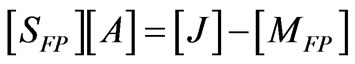
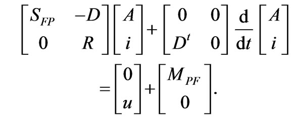
where the vector [A] represents the nodal values of vector potential, [SFP] a square matrix called stiffness matrix, [MFP] and [J] the vectors which take into account the magnetization MFP and the current density J. One can note that the matrix [SFP] is constant because the permeability νFP is constant as well. The non-linearity’s introduced by ferromagnetic materials are reported in the source term [MFP] which depends on B (i.e. A). To take into account the coupling with the external circuit of a coil made up of stranded conductors flowed by a current i, a vector [D] is introduced such that [J] = [D] i. Then, we obtain the system
 (20)
(20)
3. Genetic Algorithms
3.1. Introduction
Genetic algorithms are developed for the purpose of optimization. They allow the search for a global extremis. These algorithms are based on natural selection mechanisms (Darwin) and the genetic evolution. A genetic algorithm is changing a population of genes using these mechanisms. It uses a cost function based on a performance criterion to calculate a (fitness). Those most “strong” will be able to reproduce and have more offspring than others.
Originally, the coding of individuals was in transcribeing binary parameters to optimize to form a gene. These genes are then put together to form the chromosome. There is, however, an approach called real coding, where the functions of change and passing are rewritten to apply directly to the vector of parameters without going through the binary. We have identified a coding real, more flexible and precise. This avoids some problems due to binary encoding. The actual coding also provides a direct view of settings throughout the evolution of the population. These modified genetic operators are used in this paper as well as the improvement tools presented in [7].
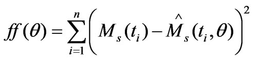
3.2. Parameters Identification Procedure
The schematic representation of the parameters identifycation procedure is shown in [8,9], the first step is the characterization of the individuals that will form the population. The individuals θ are composed by the five parameters of the J-A model (in real coding, it is not necessary to code the variables in binary representation) [6], [10]. We consider the case where the population is given by
 (21)
(21)
where each line represents an individual (a point in the optimization space), n is the generation, and np is the population size. The initial values assigned to the population are random values in the allowable range, as shown in Table 1. Each individual of the population is evaluated using the fitness between calculated and experimental results. That minimizes the fitness function given by [11]
 (22)
(22)
where  and
and represent the measured and estimated magnetization, respectively. The optimal parameter vector is obtained solving
 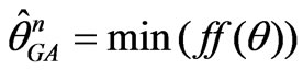 and also on a maximum allowed number of generations. Figure 1 shows the variation of the function of adaptation (fitness) according to the number generations, and Table 1 give the final results of the genetic algorithm.
3.3. The Solution Procedure
The finite Volume method is a discretization method which is well suited for the numerical simulation of various types (elliptic, parabolic or hyperbolic, for instance) of conservation laws, it has been extensively used in several engineering fields, such as fluid mechanics, heat and mass transfer or petroleum engineering [12]. Some of the important features of the finite volume
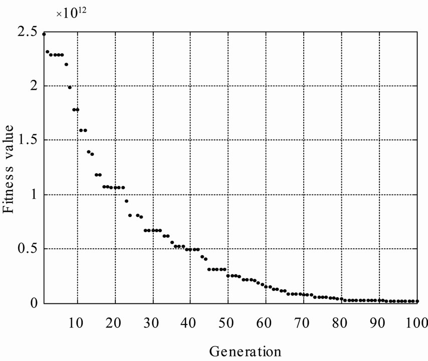
Figure 1. Evolution of the total error.
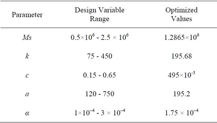
Table 1. Material parameters.
method are similar to those of the finite element method, it may be used on arbitrary geometries, using structured or unstructured meshes, and it leads to robust schemes. An additional feature is the local conservatively of the numerical fluxes, which is the numerical flux, is conserved from one discretization cell to its neighbor. This last feature makes the finite Volume method quite attractive when modeling problems for which the flux is of importance, such as in fluid mechanics, semi-conductor device simulation, heat and mass transfer.
The finite Volume method is locally conservative because it is based on a “balance” approach: a local balance is written on each discretization cell which is often called “control Volume”, by the divergence formula, an integral formulation of the fluxes over the boundary of the control Volume is then obtained. The fluxes on the boundary are discretized with respect to the discrete unknowns. The solution of the posed problem is constructed using finite Volume method. With this purpose let us multiply magnetodynamic equation (5) by function of projection βi and integrate obtained equation over domain Ω, we get
 (23)
(23)
With Βi is function of selected projection 1/r.
One can write (23) as
 (24)
(24)
After integration, this expression can be rewritten as follows
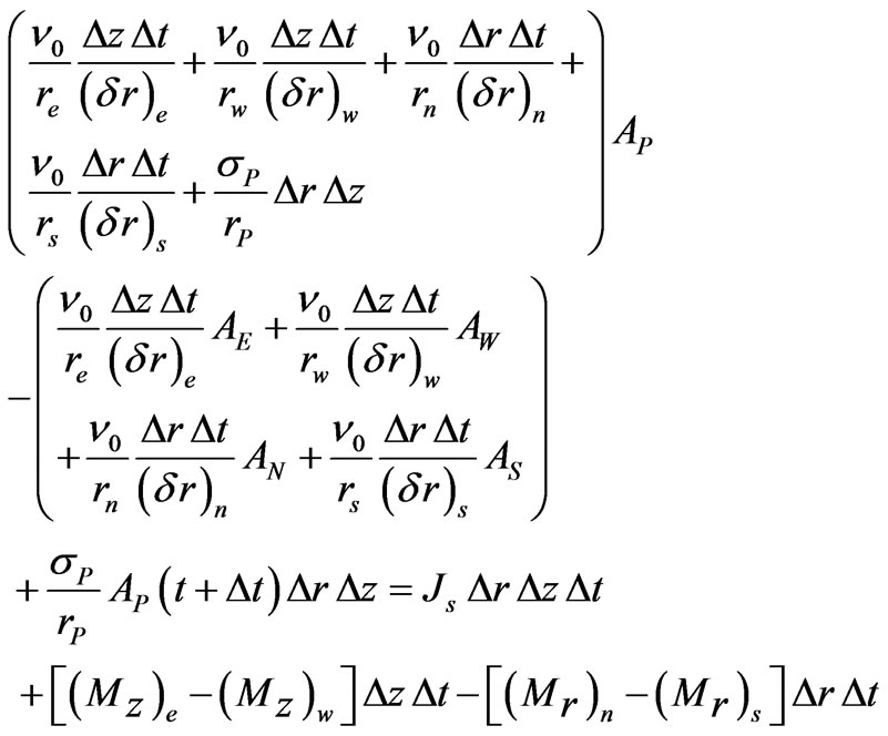 (25)
(25)
The Equation (25) discretized once is written as follows
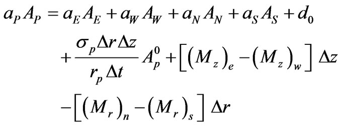 (26)
(26)
The indices P, W, N, E and S refer to the values of the nodes and indices p, w, n, e and s refer to the values of the faces of Volumes of control (See Figure 2).
The coefficients aW, aN, aE, aS and d0 is given by
 (27)
(27)
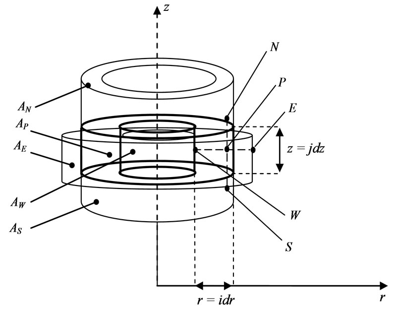
Figure 2. Control Volume in axi-symmetrical cylindrical coordinates.
Once that the various formulations in finite Volumes integrating the model of hysteresis are established a method of resolution of nonlinear problem must be chosen.
The strategy incorporated here for concurrently solving the nonlinear J-A material Equation (16), along with the spatially dependent field Equation (5), is the fixedpoint method.
The fixed-point method is the preferred method for implementing the complex mathematical material models in the finite volumes method (FVM) [1], since it is a stable method and relatively easy to implement. In the case of the Table 2, the fixed-point iteration scheme for simultaneously solving the nonlinear field Equation (5), and the J-A state model (16) steps is shown.
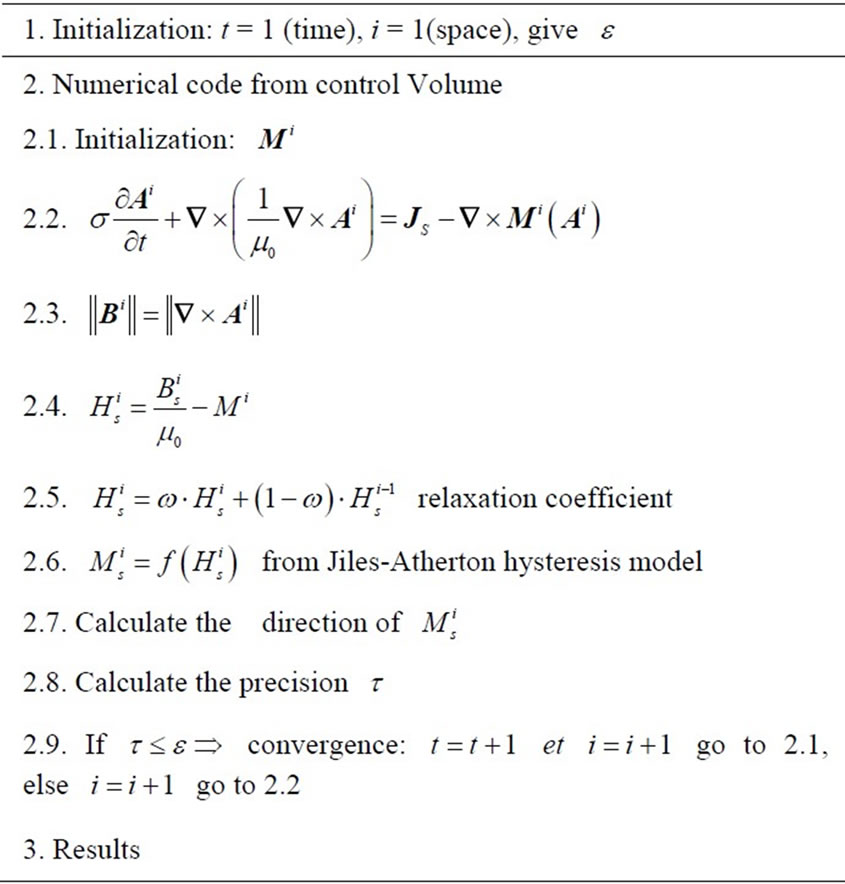
Table 2. Iterative steps algorithm.
4. Results
4.1. Measured Curves
The determination of the magnetic quality of materials rests primarily on the nature of the systems of measurement used. The evolution of the standard in the field of the characterization of material is a significant factor for the taking into account of the physical nature of magnetic materials and the conditions of their uses.
The reproducibility of measurement and the facility of handling are also factors which make it possible to choose the type of magnetic circuit to implement. Accordingly our choice is related to the realization of framework SST (Single Sheet Tester) 500 mm × 500 mm (See Figure 3) [13]. The device planned for characterization of sheets with not oriented grains must make it possible to take measurements by a simple introduction of the sample, iron silicon 3% not oriented inside a sleeve, with a perfect positioning and without deterioration of the polar faces of the magnetic circuit of closing of flux. The characterization of materials studied done by determining the following quantities expressed in terms of characterization of the frame and measuring output Voltages measured by an oscilloscope: V2, VH1, and VH2.
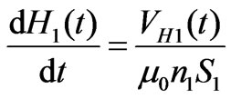
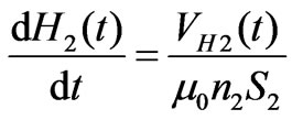
The excitation peak field, which is submitted the sample is obtained by interpolation from tensions measured at the terminals of two coils tangential H1 and H2 located at distances different from the sample
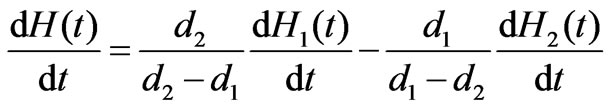 (28)
(28)
where
 (29)
(29)
and
 (30)
(30)
The magnetic induction is obtained by time integration of the V2 (t) Voltage in secondary coil measuring B by
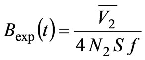 And
And 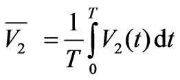 (31)
(31)
where d1, d2: Distance to sample the coil Field 1, 2 (m).
N2: Number of turns of the coil measuring B.
n1, n2: Number of turns of the coil Field No1, 2.
S: Section of the sample (m2).
S1 , S2: Surface of the coil H1, H2 (m2).
VH1, VH2: power output of the coil H1, H2 (V).
It is important to remark that the use of the inverse J-A
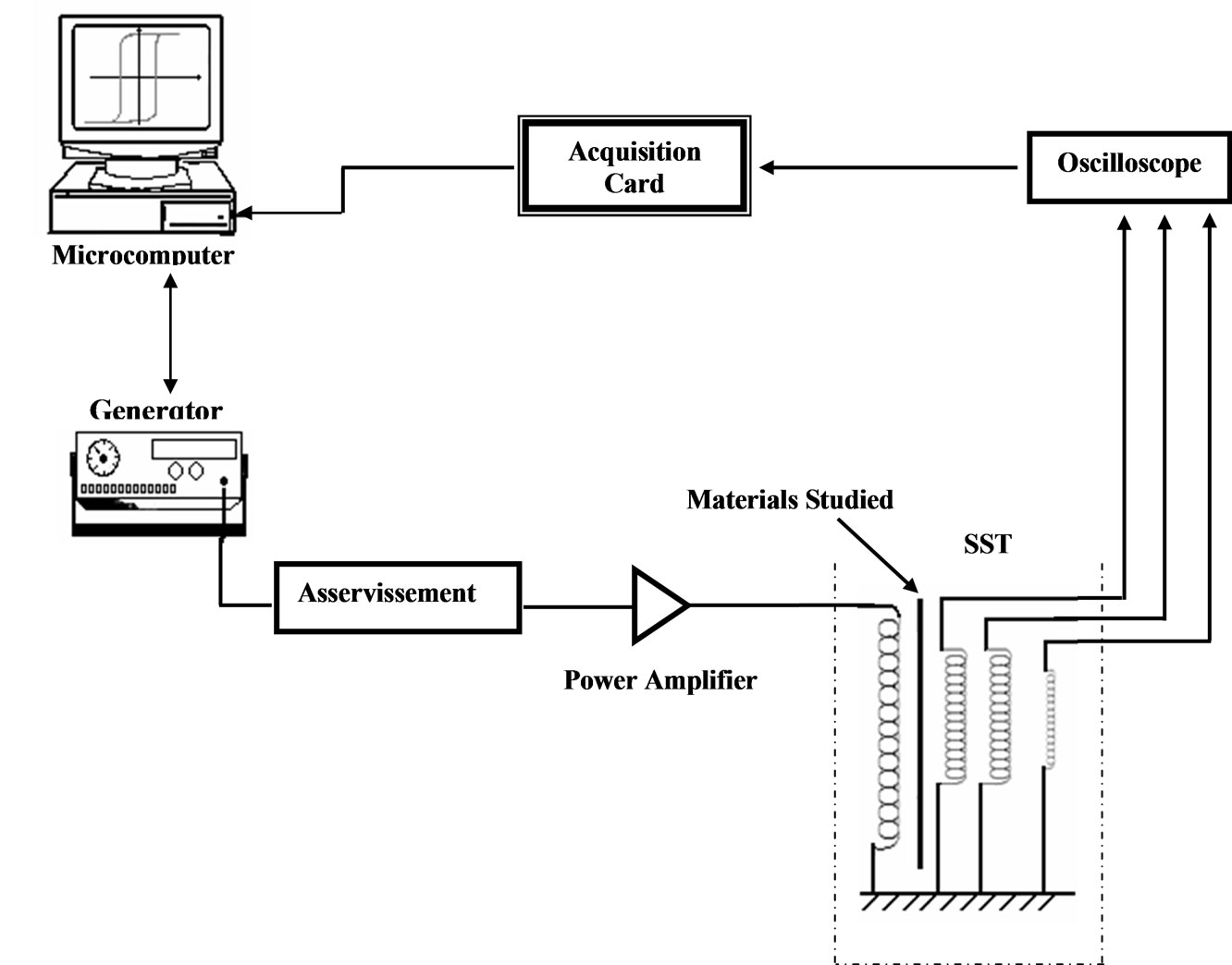
Figure 3. Single Sheet Tester (SST) 500 m × 500 m.
model for the parameters identification has an additional advantage compared with the original model: the input of the inverse model is the magnetic induction waveform. Since the magnetic induction is obtained from integration, it is naturally filtered, with fewer oscillations than those of the magnetic field waveform. The noise present in the field waveform brings additional difficulties to the parameters identification procedure. The obtained set of parameters is valid for models, original and inverse, allowing good agreement between measured and calculated data [6].
4.2. Comparison with Simulation
The test consists of a cylinder ferromagnetic with a length of 40 cm and 10 cm diameter characterized by a cycle of hysteresis (Ms = 1.2865 × 10⁶, k = 195.68, c = 495 × 10–3, a = 195.2, α = 1.75×10⁻⁴), the cylinder is surrounded by a coil of the same length traversed by a stream of density J = 105A/m2.
The drivers which constitute the inductor have a diameter D = 1 cm and 50 cm length. The gap is E = 2 cm. The geometry of the system studied, it presents two symmetries, the first axially (oz) and the second according to the plan (or). We can then consider magnetic problem in a cylindrical coordinate system, a quarter of domain. For a numerical modeling the theoretical limits (with infinite, A = 0) are brought back to a finite distance which can vary according to the desired precision. In this study, these limits were fixed at a distance L = 50 cm of the studied device. The boundary conditions associated with the magnetic equation are the conditions of Neumann  and the conditions of the Dirichlet A = 0 of representing on Figure 4.

Figure 4. Field of study of the axi-symmertical problem with the boundary conditions.
We defined in these geometry four points of reference on which we will determine the forms of wave of the magnetic potential vector. While being based on the system of axis (r, z) defined in Figure 3, the coordinates of these points are defined like: P1 (2.5, 2) cm, P2 (18, 5) cm, P3 (10, 4) cm and P4 (5, 6) cm.
Figure 6 shows, for an operation frequency of 50 Hz, the experimental and simulated field curves of this material FeSi 3% when submitted to a 1.52 T peak value sinusoidal induction.
For the validation of the parameters obtained, one superimposed on the Figure 5, the cycle experimental and the cycle of simulation obtained starting from the identified parameters. This superposition shows the degree of
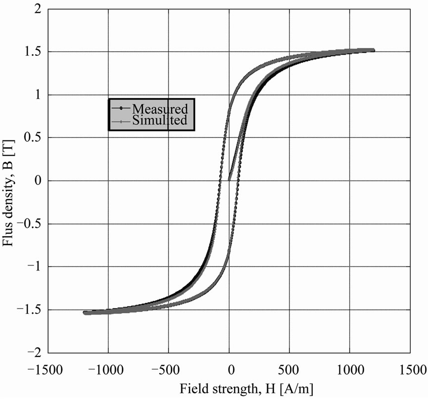
Figure 5. Measured and calculated B (H) loops at 50 Hz.
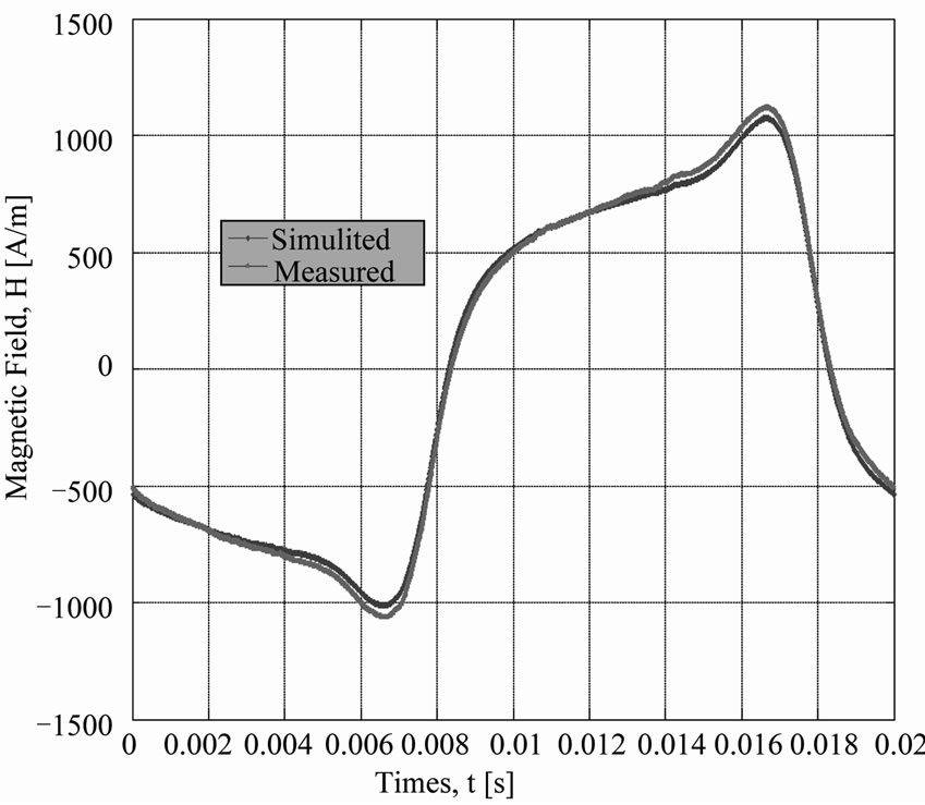
Figure 6. Field measured and modeled at 50 Hz.
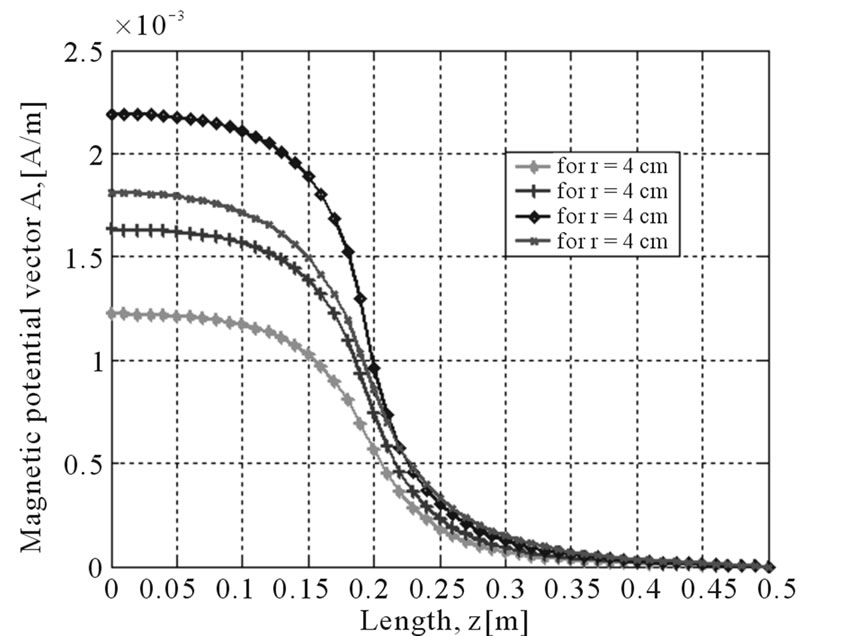
Figure 7. Axial variation of the magnetic potential vector A.
accuracy of the cycle identified by genetic algorithm.
Additional resultants are given in Figure 7, where the axial variations of potential vector magnetic A. One notices well that the value of A is maximal on the level of the center of the inductor then decreases gradually until being cancelled in extreme cases of the field of study.
5. Conclusions
In this work, a finite Volume-based transient simulation method for investigating hysteresis effects using the J-A scalar hysteresis model has been extended to 2-D problems. The identification of the parameters Jiles-Atherton model is a difficult process with to realize, but the use of the techniques of optimization by genetic algorithm makes it possible to free this difficulty. Results obtained by applying our model to the axisymmetric magnetodynamic device based on an inverse Jiles-Atherton model and a differential reluctivity has good performances with regard to numerical convergence and gives very satisfactory results on an SST’s frame. In the near future, the use of a dynamic model of magnetic hysteresis to study the behavior of material in the systems at high frequentcies and the application to other devices will be undertaken.
REFERENCES
- H. L. Toms, R. G. Colclaser and M. P. Krefta, “Tow Dimensional Finite Element Magnetic Modeling for Scalar Hysteresis Effects,” IEEE Transaction on Magnetics, Vol. 37, No. 2, 2001, pp. 982-988. doi:10.1109/20.917181
- N. Sadowski, N. J. Batistela, J. P. A. Bastos and M. Lajoie-Mazenc, “An Inverse Jiles-Atherton Model to Take into Account Hysteresis in Time-Stepping Finite-Element Calculations,” IEEE Transaction on Magnetics, Vol. 38, No. 2, 2002, pp. 797-800.
- D. C. Jiles and D. L. Atherton, “Theory of Ferromagnetic Hysteresis,” Journal of Magnetism and Magnetic Materials, Vol. 61, No. 1-2, 1986, pp. 48-60. doi:10.1016/0304-8853(86)90066-1
- K. Chwastek, “Description of Henkel Plots by the Magnetization-Dependent Jiles-Atherton Model,” Journal of Magnetism and Magnetic Materials, Vol. 322, No. 2, 2010, pp. 214-217. doi:10.1016/j.jmmm.2009.08.035
- K. Chwastek and J. Szczygłowski, “An Alternative Method to Estimate the Parameters of Jiles-Atherton Model,” Journal of Magnetism and Magnetic Materials, Vol. 314, No. 1, 2007, pp. 47-51. doi:10.1016/j.jmmm.2007.02.157
- J. V. Leite, S. L.Avila, and others, “Real Coded Genetic Algorithm for Jiles-Atherton Model Parameters Identification,” IEEE Transaction on Magnetics, Vol. 40, No. 2, 2004, pp. 888-891. doi:10.1109/TMAG.2004.825319
- J. A. Vasconcelos, J. A. Ramirez, R. H. C. Takahashi, and R. R. Saldanha, “Improvements in Genetic Algorithms,” IEEE Transaction on Magnetics, Vol. 37, No. 5, 2001, pp 3414-3417. doi:10.1109/20.952626
- P. R. Wilson, N. Ross, and A. D. Brown, “Optimizing the Jiles-Atherton Model of hysteresis by a Genetic Algorithm,” IEEE Transaction on Magnetics, Vol. 37, No. 2, 2001, pp. 989-993. doi:10.1109/20.917182
- B. Gallardo, D. A. Lowther, “Some Aspects of Niching Genetic Algorithms Applied to Electromagnetic Device Optimization,” IEEE Transaction on Magnetics, Vol. 36, No. 4, 2000, pp.1076-1079. doi:10.1109/20.877627
- K. Chwastek and J. Szczyglowski, “Identification of a Hysteresis Model Parameters with genetic Algorithms,” Journal of Mathematics and Computers in Simulation, Vol. 71, No. 3, 2006, pp. 206-211. doi:10.1016/j.matcom.2006.01.002
- L. A. L. Almeida, G. S. Deep, A. M. N. Lima and H. Neff, “Modeling a Magnetostrictive Transducer Using Genetic Algorithm,” Journal of Magnetism and Magnetic Materials, Vol. 266-230, No. 2, 2001, pp. 1262-1264.
- S. V. Patankar, “Numerical Heat Transfer and Fluid Flow,” Hemisphere Publishing Corporation, Washington, 1980.
- T. L. Mthombeni, “Improved Lamination Core Loss Measurements and Calculations”, Ph.D. Thesis, Clarkson University, Potsdam, 2006.