ABSTRACT

The investigation of contaminated areas in fractured aquifers represents a great technical challenge, due to the frequent conditions of heterogeneity and anisotropy of these environments, which often make it difficult to identify and predict pathways of subsurface contamination. This work aims to contribute to the development of this subject, through the presentation of the results of an investigation in which geophysical logging tools and straddle packers were used, which allowed the development of a more suitable hydrogeological conceptual model of the study area. Two boreholes were drilled and geophysical logging (gamma, caliper and high resolution acoustic televiewer) were used for the geological-structural characterization of the aquifer. Heatpulse flowmeter and straddle packers were then used to obtain data on hydraulic potentials and flows and for the collection of discrete water samples for chemical analysis. Two types of gneiss rocks were identified below the weathering zone (thickness >30 m), one with predominance of mafic bands, more weathered and with a higher fracture density, up to 65 m, and another deeper one, with the predominance of felsic bands. Seven groups of fractures were defined, being those of Group 1, with low dip angles, the most frequent and important for flow until 65 m, and Group 2 (N to NE-SW with high dips to W and NW) more frequent in deeper felsic gneisses. Downward hydraulic potentials were identified down to 65 m and upward potentials from the bottom up to 65 m. A hydraulic test allowed identifying the occurrence of hydraulic connection between the shallow weathering zone and the underlying fractured aquifer.

Keywords:

Fractured Aquifer, Contaminated Areas, Conceptual Model

1. Introduction

In situations of aquifer contamination, some fundamental questions that need to be addressed for the proper management of the environmental problem are: where is groundwater moving to? what are their velocities and flow rates? how are the contaminants being transported? The answers to these questions are usually obtained through the consolidation of geology, hydrogeology and contamination information and represented in a conceptual model of the contamination of the area of environmental interest.

Although all terrains exhibit particular geological complexities, cases of contamination of fractured aquifers, especially when contaminants are chlorinated organic compounds, represent even greater challenges for the definition of the conceptual model, given its generally high heterogeneity and anisotropy, which provide high complexity and many uncertainties in defining the paths and rates of the groundwater flow.

In general, the techniques and approaches used for investigation in fractured aquifers are more complex than those conventionally used for aquifers of primary porosity. Borehole drilling with the recovery of coreholes, associated with the use of different geophysical logging techniques, discrete hydraulic tests with straddle packers and the installation of multi-level monitoring wells of different designs are techniques frequently used in such investigations. The combined use of all these techniques is being developed in recent years through a methodology called Discrete Fracture Network (DFN) [1] [2] . In general, the costs associated with drilling and in-depth investigations, in addition to the complexity, heterogeneity and variability of fracture networks, are some of the factors that make it difficult to thoroughly characterize contamination in fractured aquifers.

This work aims to contribute to the development of the subject through the presentation of the results of an investigation of a contaminated area in a fractured aquifer located in a context of a tropical humid climate, where geophysical logging tools (caliper, natural gamma, high resolution acoustic televiewer and heatpulse flowmeter) and straddle packers have been used in two boreholes to develop a more suitable hydrogeological conceptual model of the site.

The combined analysis of the geophysical logging methods assists in the interpretation of the constructive conditions of the borehole or well, the identification of the types of rocks, stratigraphy and lithological contacts, the characterization of the main groups of fractures, their geometrical properties (position in space, frequency, interconnectivity) and the evaluation of the preferential paths of groundwater and pollutants [3] [4] . The use of these methods began more than 30 years ago [5] [6] and recent studies indicate that they are quite efficient in the study of fractured aquifers [7] [8] [9] . The use of the heatpulse flowmeter helps to define the direction and velocity of vertical component of the water flow in the borehole, which can be used to obtain hydraulic parameters of transmissivity of fractured aquifers [10] [11] [12] . The definition of the hydraulically active zones with the heatpulse flowmeter is of great interest because they determine the discrete depths in which hydraulic tests and the collection of water samples with straddle packers may be performed. The use of straddle packers in fractured aquifer investigations is presented by a series of authors [13] - [18] . The combination of some of the geophysical logging techniques and straddle packers were employed in this work and the results are presented below.

2. Study Area

2.1. Geology and Hydrogeology

The industrial area is located 90 km northwest of the city of São Paulo, southeast Brazil. Geologically, it is located east of the Paraná Basin, between the Valinhos (ZCV) and Campinas (ZCC) shear zones, in the Itapira Complex [19] , which belongs to the Tocantins Province [20] . The main outcropping rocks in the area are gneisses.

Based on field observations and considering the classification of soils proposed by Vaz [21] , three geological units were locally defined: the first corresponds to a relatively homogeneous and isotropic eluvial soil, composed of a clay-silty material of reddish brown color. Locally, a layer of landfill with sandy portions was also verified on the first horizon. The other two underlying units were classified as weathered bedrock soil and slightly weathered bedrock (gneiss) (Figure 1).

The weathered bedrock soil is a soft material resulted from the weathering of the gneiss rocks, being composed of a silt-clayey to a silt-sandy material, with a marked presence of micaceous minerals and quartz crystals. In general, this medium exhibits behavior similar to that of a primary porosity aquifer, but with zones of greater or lesser resistance associated with structures of the parental gneiss rock, which may create preferential flow paths in the water table aquifer.

The water table aquifer is represented by this weathered bedrock soil, where the hydraulic conductivities vary from 1.29E−7 to 4.28E−7 m・s⁻¹ [22] . In this aquifer, no significant differences in hydraulic heads were observed in the vertical direction, especially among the multilevel monitoring wells installed between the depths of 3.8 and 36.9 meters.

The flow direction of the groundwater in the water table aquifer presents a predominant horizontal component to the northeast, towards the stream located at the northern boundary of the industrial unit (Figure 2). In the central portion of the area, the flow presents radial characteristics associated with the topography of the region.

The slightly weathered gneiss rock has a grayish color and a medium to fine grain size. The logs of the boreholes performed in the area and surface geophysical

survey data indicate that the top of the hard rock is present at shallower depths in the west portion of the area (between 16 and 34 m) and deeper in the eastern portion. The fractured structures that are favorable for the water flow are those of NNE and those of NE to ENE directions, which are present in the rocks located west of the Campinas Shear Zone (ZCC) and between the Valinhos (ZCV) and Campinas shear zones [23] . In the gneisses and granites east of the ZCV, the most favorable structures exhibit the opposite direction: NW, WNW and NNW.

2.2. Environmental Problem

The improper use of chlorinated solvents in the past has led to contamination of the shallow aquifer within the plant. Trace concentrations of chlorinated hydrocarbon compounds were detected in the supply well P6, located about 100 m from the defined source of contamination zones (Figure 2). The site neighborhood had no public water supply system at that time and water supply was exclusively performed by pumping private wells that extracted water from the fractured bedrock aquifer.

Chlorinated organic compounds are often used in a variety of industrial processes. Many of these compounds are highly toxic and, even at low concentrations in the soil, water or atmosphere, can contaminate large areas, posing risks to human health and the environment [24] [25] . In the study area, chlorinate

solvents were used as degreasers in the cleaning of parts and equipment, and a single source area of contamination was not possible to be identified, since these activities happened in different places in the industrial unit.

Environmental investigations began in 2006 and resulted in the installation of 59 monitoring wells at three depths in the water table aquifer, for horizontal and vertical delimitation of the contamination. Two sources of contamination were identified in the shallow aquifer, named in this study as Area 1 and Area 2 (Figure 2), where the compounds tetrachloroethene (PCE), trichloroethene (TCE), cis-1,2-dichloroethene (cis1,2DCE), trans-1,2-dichloroethene (trans1,2DCE), 1,1-dichloroethene (1,1DCE), 1,1-dichloroethane (1,1DCA) and vinyl chloride (VC) were detected in groundwater.

In Area 1, concentrations of more degraded compounds predominate as cis1,2DCE and vinyl chloride. Concentrations of TCE are small and observed at the deepest level of the aquifer. In Area 2, the TCE shows the highest concentration and distribution in the area. Concentrations of degraded compounds, such as cis1,2DCE and vinyl chloride, are not significant in Area 2. Local concentrations of PCE, 1,1DCE and 1,2DCA are also observed.

Taking into account the contamination scenario presented and the detection of chlorinated compounds in the deep supply well P6, installed in the fractured aquifer, it was necessary to adopt different investigation techniques to characterize the fractures and to build an initial conceptual model of flow and transport of contaminants in the aquifer, which would be the basis for the subsequent stages of environmental management and remediation.

3. Method

3.1. Drilling Boreholes and Logging Data

An organization of information from previous works was carried out initially, such as aerial image interpretations, surface geophysical surveys and local field geological mapping. This stage was important for the identification and characterization of the main rocks and structures that occur in the region, assisting in the planning of the field stages and in the choice of the investigation methods used.

For the investigation of the fractured aquifer, two boreholes were drilled in locations close to the plumes of contamination of the shallow aquifer (Figure 2), followed by the installation of two deep monitoring wells (PP-01 and PP-02). Two drilling methods were used in each borehole: the hydraulic-rotary method to drill the soft weathered bedrock until the top of the hard rock; and the rotary air percussion drilling method, to drill the hard gneiss rock. The borehole walls were cemented and cased with a 6” carbon steel casing along the soft weathered bedrock to prevent crumbling and infiltration of the contaminated water from the shallow portions of the aquifer. As a result, well PP-01 had a total depth of 78.0 m, being the first 39.5 m corresponding to the cased soft weathered bedrock. Well PP-02 had a depth of 92.0 m, with a cased portion of 30.0 m.

After the end of the drilling activities, the boreholes were filmed aiming to identify faciological variations of the local gneiss, zones of fractures and more weathered intervals. The shooting tool used is composed of two independent front and side view cameras that can be operated in stationary or rotating mode. Additionally, a caliper coupled to a probe and constituted by three articulated rods was used to record the diameter of the boreholes. Wall diameter variations provided information on possible fractures or zones of rock weakness.

Acoustic imaging and natural gamma logging techniques were used in both boreholes through a Robertson Geologging probe with vertical resolution up to 1 mm. The High Resolution Acoustic Televiewer (HRAT) logging was performed in the boreholes in order to determine the precise oriented-location of the main fracture zones and identify the different families of fractures intercepted by the boreholes, their directions and dips. Subsequently, it was sought to correlate the fractures observed in the boreholes with surface-discontinuities mapped in previous studies.

The loggings of the natural groundwater flow inside the boreholes were performed with the use of a flowmeter, aiming to determine the flow velocity and the main inputs and outputs of groundwater in the boreholes through the identified fractures. The flowmeter model used was a Robertson Geologging one, which allowed readings with a resolution of 0.001 m・min⁻¹ in up to 30 seconds after the emission of the heat pulse. At least three measurements at each point were performed, located before and after zones of fractures selected. The fractures of interest are those that presented evidence of openness, having a greater probability of flow.

3.2. Interpretation of the Structural Data

All the data obtained with the logging activities were inserted and interpreted in WellCad v.5 software. The features identified with HRAT were traced and classified according to their degree of uncertainty in Fractures (traced in blue) and Possible Fractures (traced in pink). Some foliation measurements were also taken (traced in green) at each of the analyzed points. The structural data obtained (fracture attitude) are presented in the Clar compass notation (strike and dip angle) and were first compiled in spreadsheets and later imported by DIPS software v.5, analyzed in stereograms, density diagrams and histograms, to define the different groups of fractures present.

For the analysis of the fractures density and spacing, the method developed by Terzaghi [26] and adapted by Pino [27] was used to adjust the density of fractures intercepted by the borehole. This correction is necessary since the fracture data are affected by the bias of the drilling orientation and the apparent spacing of the fractures, related to the angle (α) that the fracture makes with the borehole axis. In this analysis, the values corrected for fractures with α angle greater than 20˚ and absolute values for the other fractures were corrected, thus ensuring that all observed features are considered. The main groups or fracture families of the rock were characterized to help defining the main zones of water flow and contaminants.

3.3. Straddle Packers

After the interpretation of the data obtained with the borehole logging activities, water samples were collected from fractures of the crystalline aquifer with the use of straddle packers. This equipment isolates sections of the borehole, allowing the obtainment of water samples at discrete intervals. The packers used consist of two inflatable cylindrical rubbers, coupled to a steel main support rod (Figure 3). The rubbers work as bladders and are inflated to the desired depth with the use of air compressors or gas cylinders, isolating the desired interval.

A low-flow bladder pump was used to conduct the sampling activities, being inserted inside the main support rod, which is hollow and has opening only in the filtering portion between the packers, allowing the water to enter the sealed portion into the pump. In this way, it was possible to carry out the cleaning activities of the pump and exchange hoses between the sampling events, avoiding cross contamination by the sampling equipment. Three sampling points were selected in each borehole.

Sampling activities comprised the following steps: (1) water level measurement; (2) positioning the pump and packers at the desired depth, starting from the bottom of the borehole; (3) filling the straddle packers and waiting for

approximately 30 min for hydraulic head stabilization, prior starting the pumping; (4) purging the water within the insulated range for approximately 30 min; (5) measurement of hydraulic heads and physical-chemical parameters for every 5 min until stabilization; and (6) collection of groundwater samples for the analysis of volatile organic compounds (VOC) by GC/MS (USEPA method 8260B). During the sampling activities, the hydraulic heads in the isolated interval by and above the packers were monitored, in order to evaluate the efficiency of the insulation.

After the evaluation of the results of the chemical analysis, the work continued with the installation of a conventional monitoring well at each borehole, in order to allow the continuity of the monitoring in the fractured aquifer. The filters were positioned where the highest concentrations of organic compounds were detected (Figure 4). A pumping test was then conducted in the deep supply well P6, in order to evaluate the hydraulic connectivity of the deep fractured aquifer and the water table aquifer. Hydraulic heads of three monitoring wells installed in the water table aquifer were monitored during the pumping test.

4. Results and Discussion

4.1. Borehole Geological Description

The geological logs of the boreholes and the design of the monitoring wells

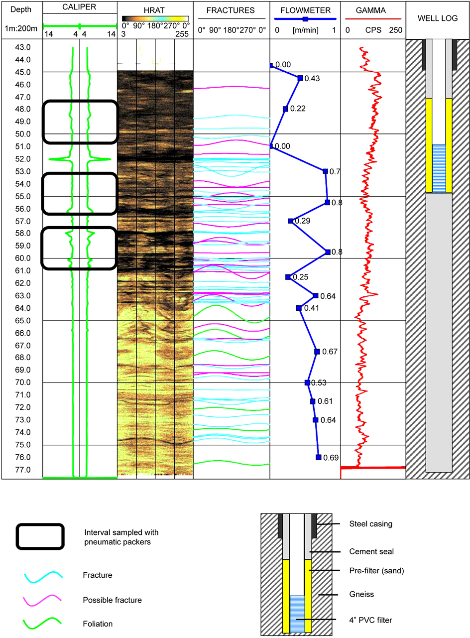
PP-01 and PP-02 are presented in Figure 4. The data obtained by the caliper, gamma and HRAT logging were imported by WellCAD v.5 software, handled and analyzed together with the filming and other data collected in the field stage. These are presented in Attachment 1.

The results indicated the occurrence of two faciological zones in the gneiss rock. From the top of the rock (base of the weathered bedrock soil) to the average depth of 65.0 m, in both boreholes, a dark gray gneiss predominates, where minerals such as biotite, hornblende, amphibole and alkali feldspar are present. After the depth of 64 m in the PP-01 and 65 m in the PP-02, the gneiss is light, of whitish color, formed essentially by quartz, alkali feldspar and plagioclase.

At both boreholes, the gneiss rock is intensely fractured, especially in the uppermost dark gneiss portion, near the contact of the weathered rock soil with the top of the fresh rock. In this portion, the gamma ray logs presented higher values, related to the greater presence of clay minerals in the rock. In depth, the rock presents a smaller number of fractures and the presence of quartz and plagioclase can also contribute to the reduction of gamma rays values (Attachment 1).

In PP-01, variations associated with the occurrence of large fractures were recorded by caliper logging between 45.0 and 61.0 m (Attachment 1). The natural gamma logging in PP-01 showed average values between 120 and 140 cps to the approximate depth of 64.0 m, and smaller values, in the order of 80 cps, after this depth. In PP-02 (Attachment 1), fractures with larger apparent openings are spaced and present throughout the profile, with more weathered zones located closer to the ground surface. The values of the gamma radiation range from 120 to 180 cps to the depth of approximately 65.0 m, when there is a reduction to values between 40 and 100 cps.

4.2. Structural Analysis

Based on the HRAT data, the fracture and foliations features were defined and the depth and attitude data (strike and dip) were treated in rose diagrams, histograms and stereograms, helping to define the different groups. In the stereograms, the dubious features were characterized as “Possible Fractures” and represented in blue dots, in order to facilitate the evaluation of their importance and coherence with respect to “Fractures”, represented in red and used primarily for the separation of the main groups. Foliation measurements are shown in black. Figure 5 and Figure 6 present the data obtained for PP-01.

More than 30% of the features observed in PP-01, including foliation measurements, present N-S main direction, ranging from N0-25E. The section between 52 and 64 m presents the largest number of fractures. It is recalled that the boreholes are vertical, which makes it difficult to visualize possible existing high angle fractures, whose quantification may be underestimated. Nevertheless, the number of fractures identified parallel to the foliations, with subvertical dips, is significant. It is possible to identify at least five groups of major fractures in PP-01, described below.

Group 1: Sub-horizontal fractures, striking predominantly N45W to N30E and dipping less than 40˚, preferably to W and with small variations to SW or NW. The fractures present a random distribution, they are apparently open and occur mainly in the most weathered dark portion of the gneiss. It is the group of greater density, smaller average spacing and with preferential occurrence in the upper portion of the rock massif.

Group 2: Structures parallel to the foliation, striking N0-22E (vertical) with high dip (>60˚) to W. This is the second group of major importance. The fractures are observed from 58 m depth and are more expressive in the light gneiss portion, below 64 m. Due to high dip, group 2 fractures were not considered in the Terzaghi correction, which indicates that the number of features observed may be underestimated.

Group 3: E-W fractures predominate, dipping >45˚ preferably to S. Fractures of this group are more spaced throughout PP-01. Only the features observed dipping 45˚ to 70˚ are corrected by the Terzaghi method, according to Figure 5.

Group 4: NE-SW fractures, dipping 60˚ - 70˚ to SE. Only three representative features of this group were registered at depths of 54, 72 and 73 m, but the group becomes more expressive after the application of the Terzaghi correction.

Group 5: E-W to WNW fractures, dipping >55˚ to N. These features are observed only in the upper portion of the rock, up to 55 m depth and only fractures dipping 55˚ to 70˚ are influenced by the Terzaghi correction.

Structural data obtained for PP-02 are presented in Figure 7 and Figure 8. 40% of the observed features are NE-SW, represented mainly by fractures of Groups 1, 2 and 4. The foliation measurements also show this strike. The intervals of 35 to 43 m and 62 to 73 m represent zones intensely fractured, favorable to the groundwater flow. The fractures with the largest openings show dips of <40˚ and the deepest portion of the borehole presents the largest number of fractures, apparently with no openings.

In PP-02, fractures of Group 1 are characterized by a dispersed strike and low

to medium dip. However, NNE-SSW fractures dipping WNW predominate. It is the group with the highest density and lowest spacing, and it was possible to identify two areas where the density distribution is remarkable: the subgroup 1-a, characterized by low dip (up to 35˚); and subgroup 1-b, with a little higher dips, between 40˚ and 60˚. As in the PP-01 borehole, Group 1 fractures in PP-02 occur more frequently in the upper dark-grey portion of the gneiss, but scattered fractures were observed until the bottom of the borehole. The application of the Terzaghi correction was more significant in the subgroup 1-b.

Group 2 fractures in the PP-02 are N-NE (N15-45E), dipping W to NW with higher angles, between 60˚ and 85˚. In stereograms with density contours drawn for the different depths (Figure 7(c), Figure 7(d)), it is clear the separation of the fractures of groups 1 and 2, since the two groups generally have the same strike, but different dips. The fractures of Group 2 are parallel to the foliation and, although they occur throughout the borehole, they are more frequent in the deepest portion of the borehole PP-02.

In a smaller number, Group 3 fractures are N60 - 80W, dipping >55˚ to SW, predominantly occurring in the upper dark-grey gneiss. Group 4 fractures are NE-SW, dipping 55˚ - 75˚ to SE. Group 5 fractures were not identified in this borehole; however, two new fracture groups were defined: Group 6 are N10-30W/50-70SW and Group 7 EW/40-50N.

4.3. Groundwater Sampling Using Straddle Packers

Based on the fractures structural data gathered previously, three discrete intervals in each borehole were selected for collecting groundwater samples, through the use of straddle packers. The selected depths and the results of VOC concentrations are presented in Table 1.

In the PP-01 borehole, the groundwater sampling was conducted in the upper dark grey gneiss, which is more fractured. The VOCs analysis detected concentrations of the compounds 1, 1DCE, 1, 1DCA, 1, 2DCE and TCE above the

a. Cetesb 2014 corresponds to the Sao Paulo State environmental standards. b. Asl = “above sea level”. c. DCM = Dichloromethane. For other abbreviations, see item 2.2.

environmental standards in PP-01. The compounds PCE and toluene were also detected.

Concentrations of 1, 1DCA, 1, 1DCE, toluene and TCE were detected below standards in the PP-02 borehole. Considering the similarity between the concentrations of the compounds detected and the possibility of water samples represent mixtures of different depths during sampling, due to interconnection between the fractures in PP-02, it was not possible to confirm which of the depths sampled shows the highest concentrations of the contaminants.

4.4. Evaluation of Groundwater Hydraulic Potentials and Flow

The PP-01 borehole exhibited the main flow variations (water inlets and outlets) associated with the first 20 meters of rock (from 45 to 65 m bgs), where Group 1 fractures predominate. The highest observed velocities were 0.82 m・min⁻¹ at 55.5 m and at 59.5 m depth (Attachment 1). There is also an expressive loss of water velocity between 53.0 and 51.0 m, reaching 0 m/min. This variation can be attributed to the exit of water from the borehole through fractures identified at 52.0 m depth, which walls are weathered and with an apparent opening of 0.5 cm, the largest in PP-01 associated to Group 1.

During the sampling activities, the hydraulic heads measured between the packers after head stabilization (Table 1) indicated a slightly vertical downward potential for the groundwater flow in the fractured aquifer (9 cm of hydraulic head variation from 47.2 to 62.1 m). However, variations in hydraulic potentials above the packers were observed during pumping at these three sampling depths, indicating that it was not possible to completely isolate the sampled intervals, even with the increase in the filling pressure of the packers. This interference may be due to the wall roughness of the borehole or the connection between the fractures in the rocky massif, especially those of high dip.

In PP-02, the fractures with larger apparent openings are spaced along the borehole, however, the higher flow velocities were also observed in the in the upper dark grey gneiss. The average velocities obtained in PP-02 were higher than those found in PP-01. The highest flow velocities were observed in the intervals between 32.0 and 38.1 m and from 61.0 to 62.0 m (Attachment 1). In the first section, Group 1 fractures predominate with dips <60˚ and the maximum measured velocity was 1.20 m/min. In the second interval, fractures of Group 3 and 4 predominate and the flow velocity was measured as 1.02 m/min.

The hydraulic heads measured in the borehole PP-02 above the packers did not change during the pumping for groundwater sampling at each depth, whereas, in the section between the packers, it was possible to observe a subtle variation, indicating a greater efficiency in the isolation of the sampled portion.

The hydraulic heads measured between the packers after head stabilization (Table 1) indicated a slightly vertical downward potential for the groundwater flow from level A to B (46 cm of hydraulic head variation from 36.2 to 64.3 m bgs) and a light upward potential for groundwater flow from level C to B (6 cm of hydraulic head variation from 88.2 to 64.3 m bgs).

4.5. Monitoring Wells and Hydraulic Tests

After the groundwater sampling activities with the straddle packers, monitoring wells were installed at the intervals where the greatest velocity variations measured by the flowmeter and the highest VOC concentrations verified by sampling with the packers were verified. In the monitoring wells, the filter was installed in the depths of 50.8 to 54.8 m in PP-01 and from 35.3 m to 38.3 m in PP-02. In both wells, the rest of the boreholes underneath the filter depths was cemented.

After the well completion, they were developed and then recovery hydraulic tests were conducted in both wells. The analyzed intervals correspond to the permeable zone of the formation where the filters and prefilters were installed. Data were interpreted using the Hvorslev method [28] . The hydraulic conductivities obtained are 1.45E−6 m/s for PP-01 and 5.34E−7 m・s⁻¹ for PP-02.

A pumping test was conducted in the deep supply well P6, located 100 m far from the plume of contamination of the shallow aquifer in Area 1 (Figure 2), in order to evaluate the hydraulic connectivity of the deep fractured aquifer with the shallow water table aquifer of the industrial unit. During the pumping period, hydraulic heads of three monitoring wells installed in the water table aquifer were monitored: monitoring well MW 09B (109 m far from P6), MW 54 (17 m far from P6), and MW 34 (55 m far from P6), besides the new monitoring well PP-01 (91 m far from P6), with filter installed in the fractured aquifer (Figure 2). The pumping was carried out at a constant flow rate of 2.1 m³・h⁻¹ and lasted 11 hours and 20 minutes. Figure 9 shows the variation of water level depths measured in each of the monitoring wells.

Only monitoring well 54, which is the closest to the pumping well P6, showed a clear influence of the pumping, with a hydraulic head variation of 0.37 m. MW 54 presents a depth of 29.5 m and is installed in the water table aquifer, in the weathered bedrock and close to the contact with the hard fractured rock. Despite the short pumping time period, the test made it possible to confirm the connection between the aquifers and the rapid influence of the pumping of the deep supply well in the shallow wells, indicating that the fractures in the rock are hydraulically connected with the shallow aquifer at the base of the weathered bedrock.

5. Hydrogeological Conceptual Model

Figure 10 presents the hydrogeological conceptual model of the study area. The weathered bedrock of the gneiss rock is represented by a silt-clayey to silt-sandy material, with intercalations of quartz veins and clayey portions with discontinuities, which characterize it as a heterogeneous and anisotropic medium. The boreholes where located in the highest portions of the terrain and reached the top of the hard rock at 39.5 m in PP-01 and 30 m in PP-02.

The fractured aquifer is composed of two types gneisses below the weathering

zone, one with predominance of mafic bands and other with felsic bands. From the top of the rock to the mean depth of 65 m, the mafic portion of the gneiss predominates. This interval is quite fractured and weathered. The predominance of felsic bands in the gneiss, mainly composed of quartz, alkali feldspar and plagioclase, occurs from 65 m.

Fractures with larger apparent openings and larger flow variations, verified in both boreholes, are generally those of low to medium dip, located in the first 25 meters of the weathered rock. They have a varied but predominant N to NE strike and were classified as Group 1. Group 2 fractures, with high dip angle, parallel to the foliation, are N to NE-SW dipping to W to NW and are, in general, more expressive in depth. Group 3 fractures are found throughout the entire PP-01 and also in the mafic portion of the PP-02 and present a medium to high dip, from E-W to NW-SE.

The presence of Group 1 fractures positioned mainly in the more superficial portion of the rock, intercepting fractures of medium to high dips, mainly of Groups 2, 3, 4 and 7, help in the hydraulic connection between the water table and the fractured aquifer, contributing for the migration of contaminants to deeper zones. Previous works on the fractured aquifer dynamics of the region [19] indicate that the fractures of NE to ENE and NNE are parallel to foliation and preferentially of distensive nature, being related to the main water conducting structures in the gneisses.

Hydraulic potentials measured during groundwater samplings with the straddle packers indicate the occurrence of a downward flow of water in the upper portion of the rock (up to approximately 65 m) and an upward flow in the deepest portion. Despite the natural downward flow from the fractures of the upper portion of the rock, the influence of the supply wells pumping favored a faster migration of the plumes of contamination from the shallow aquifer into the fractured aquifer. The pumping of the supply well P6 and the declining of the water level of the well 54 is an indication of the hydraulic connection between the aquifers and the influence of the pumping of the supply wells in the shallow aquifer. Despite the similarity between the results of the chemical analyzes of the samples collected with the packers, the presence of dissolved chlorinated compounds was confirmed in both boreholes, with higher concentrations in PP-01.

When comparing the lineament traces that cross the study area with the occurrence of the contaminants observed, it is possible to identify a relationship between the compounds in the groundwater with the monitoring wells located in the same structural region, among the identified lineaments. The contamination observed in P6 is more similar to that observed in Area 2, although it is closer to the plume of Area 1. Thus, it is possible to suppose that the water flow is influenced and controlled by the existing regional structures, which may be draining groundwater regionally.

6. Conclusions

This work presents the results of the investigations carried out in a fractured aquifer for the improvement of the conceptual model of the contamination by chlorinated solvents in an industrial unit. Unlike investigations of aquifers of primary porosity, the investigations in fractured aquifers involve the application of specific techniques in a sequence of achievements, starting with the geological and surface geophysics, which are the basis for the location of boreholes. In the borehole, geophysical logging procedures are used for the geological and structural characterization of the aquifer rocks. Flowmeter and straddle packers are then used to provide information on the groundwater flow characteristics, measure hydraulic heads, hydraulic properties of fractures and collection of discrete water samples for analysis. These data are then interpreted for the design of monitoring wells. Priority is then given to the long-term monitoring of those fractures that carry a greater mass of the contaminants. In this work, not all the techniques described in the literature were used, like straddle packers for determining transmissivity of fractures, especially due to financial and time restrictions.

However, the greatest possible amount of information of this nature is important for the decision making process for the management of contaminated areas [29] , since they allow to identify if contamination exists in the fractured aquifer, where it moves to, what are the receptors to be protected, and types of intervention to be applied (e.g. the decision to stop or continue the pumping of neighboring water supply wells to avoid spreading contamination in the aquifer).

It often occurs that the complexity of fracture networks does not allow local data obtained with a single borehole to be extrapolated to the study area as a whole. Thus, the understanding of the path of contamination requires obtaining data from other borehole with the application of the maximum of proposed techniques, including the execution of more complex hydraulic tests, such as those of cross-borehole types. The minimum number of wells required for the execution of a suitable hydrogeological model depends on the importance of the properties and environmental resources to be protected, the existence of human and ecological receptors, the intensity and size of the contamination and the complexity of the geological environment. The evaluation of these variables in each case should be taken into account to define the amount of financial effort necessary to improve the conceptual model of the area of environmental interest.

Acknowledgements

The authors express special thanks to Daphne Pino, Marcos Bolognini Barbosa and Amélia J. Fernandes for their valuable contributions during the stages of fieldwork activities and data interpretation. And also to Waterloo Brasil ConsultingLtda and the anonymous industrial company that kindly authorized the use of the data for publication.

Cite this paper

Fanti, A., Bertolo, R., Vogado, F., Cagnon, F. and Queiroz, A.P. (2017) Application of Geophysical Logging and Straddle Packers for the Investigation of a Fractured Aquifer in a Contaminated Area by Chlorinated Solvents in Sao Paulo State, Brazil. Journal of Water Resource and Protection, 9, 1145-1168. https://doi.org/10.4236/jwarp.2017.910075

References

Attachment 1

PP-01 and PP-02. Two deep monitoring wells (inserting PP-01 and PP-02).

References

- 1. Parker, B. (2007) Investigating Contaminated Sites on Fractured Rock using the DFN Approach. Proceedings at the USEPA/NGWA Fractured Rock Conference: State of the Science and Measuring Success in Remediation, Maine, 150-168.
- 2. Parker, B., Cherry, J. and Chapman, S. (2012) Discrete Fracture Network Approach for Studying Contamination in Fractured Rock. AQUA mundi, Am06052, 101-116.
- 3. Keys, S. (1990) Techniques of Water-Resources Investigations of the United States Geological Survey. USGS Report, 165 p. https://pubs.usgs.gov/twri/index090905.html
- 4. Lane, J. (2002) An Integrated Geophysical and Hydraulic Investigation to Characterize a Fractured-Rock Aquifer. U.S. Department of the Interior, U.S. Geological Survey, Norwalk, 97 p. https://water.usgs.gov/ogw/bgas/publications/wri014133/
- 5. Lau, J., Auger, L. and Bisson, J. (1987) Subsurface Fracture Surveys using a Borehole Television Camera and Acoustic Televiewer: Reply. Canadian Geotechnical Journal, 24, 499-508. https://doi.org/10.1139/t87-066
- 6. Cruden, D. (1988) Subsurface Fracture Surveys using a Borehole Television Camera and Acoustic Televierwer: Discussion. Canadian Geotechnical Journal, 25, 843. https://doi.org/10.1139/t88-094
- 7. Morin, R., Godin, R., Nastev, M. and Rouleau, A. (2007) Hydrogeologic Controls Imposed by Mechanical Stratigraphy in Layered Rocks of the Chateauguay River Basin, a US-Canada Transborder Aquifer. Journal of Geophysical Research, 112, B04403.
- 8. Robinson, D., Binley, A., Crook, N. and Slater, L. (2008) Advancing Process-Based Watershed Hydrological Research using near Surface Geophysics: A Vision for, and Review of, Electrical and Magnetic Geophysical Methods. Hydrological Process, 22, 3604-3635. https://doi.org/10.1002/hyp.6963
- 9. Francese, R., Mazzarini, F., Bistacchi, A., Morelli, G., Pasquare, G., Praticelli, N., Robain, H., Wardel, N. and Zaja, A. (2009) A Structural and Geophysical Approach to the Study of Fractured Aquifers in the Scansano-Magliano in Toscana Ridge, Southern Tuscany, Italy. Hydrogeology Journal, 17, 1233-1246. https://doi.org/10.1007/s10040-009-0435-1
- 10. Paillet, F. (1995) Using Borehole Flow Logging to Optimize Hydraulic Test Procedures in Heterogeneous Fractured Aquifers. Hydrogeology Journal, 3, 4-20. https://doi.org/10.1007/s100400050249
- 11. Day-Lewis, F., Johnson, C., Paillet, F. and Halford, K. (2011) A Computer Program for Flow-Log Analysis of Single Holes (FLASH). Groundwater, 49, 926-931. https://doi.org/10.1111/j.1745-6584.2011.00798.x
- 12. Johnson, C., Mondazzi, R. and Joesten, P. (2009) Borehole Geophysical Investigation of a Formerly Used Defense Site, Machiasport, Maine, 2003-2006. USGS Scientific Investigations Report 5120, 87 p.https://pubs.usgs.gov/sir/2009/5120/pdf/sir2009-5120_text_508.pdf
- 13. Lapcevic, P. (1988) Results of Borehole Packer Tests at the Ville Mercier Groundwater Treatment Site. NWRI Contribution 88, RRB-88-92. National Water Research Institute Canada Centre for Inland Waters, Burlington, 30 p.
- 14. Novakowski, K., Bickerton, G., Lapcevic, P.V.J. and Ross, N. (2006) Measurements of Groundwater Velocity in Discrete Rock Fractures. Journal of Contaminant Hydrology, 82, 44-60.
- 15. Wahnfried, I. (2010) Hydrogeologycal Conceptual Model of the Serra GeralAquitard and Guarani Aquifer in Ribeir ãoPreto, São Paulo, Brazil. Doctoral Thesis, Institute of Geosciences, University of Sao Paulo, Sao Paulo. (In Portuguese)http://www.teses.usp.br/teses/disponiveis/44/44138/tde-07072010-163245/publico/IW.pdf
- 16. Quinn, P., Parker, B. and Cherry, J. (2011) Using Constant Head Step Tests to Determine Hydraulic Apertures in Fractured Rock. Journal of Contaminant Hydrology, 126, 85-99.
- 17. Quinn, P., Cherry, J. and Parker, B. (2011) Quantification of Non-Darcian Flow Observed during Packer Testing in Fractured Sedimentary Rock. Water Resources Research, 47, 15 p. https://doi.org/10.1029/2010WR009681
- 18. Quinn, P., Cherry, J. and Parker, B. (2012) Hydraulic Testing using a Versatile Straddle Packer System for Improved Transmissivity Estimation in Fractured-Rock Boreholes. Hydrogeology Journal, 20, 1529-1547. https://doi.org/10.1007/s10040-012-0893-8
- 19. IG-SMA, InstitutoGeológico (1993) Aids of the Geological Physical Environment to the Planning of Campinas Municipality (Brazil). Technical Report, Volume II, Sao Paulo. (In Portuguese)
- 20. Almeida, F., Hassui, Y., Brito Neves, B. and Fuck, R. (1977) Structural Brazilian Provinces. Proceedings at the 8th SBG Northeast Geology Symposium, Campina Grande.
- 21. Vaz, L. (1996) Genetic Classification of Soils and Weathered Rock Horizons in Tropical Regions. Solos e Rochas, 19, 117-136. (In Portuguese)
- 22. Waterloo Brasil (2011) Geological Study and Top of Bedrock Mapping. Technical Report, Confidential, São Paulo.
- 23. Fernandes, A. (1997) Cenozoic Tectonics of the Piracicaba River Basin and Its Application to Hydrogeology. Doctoral Thesis, Institute of Geosciences, University of Sao Paulo, Sao Paulo. (In Portuguese)http://www.teses.usp.br/teses/disponiveis/44/44133/tde-30092013-163243/pt-br.php
- 24. Pankow, J. and Cherry, J. (1996) Dense Chlorinated Solvents and Other DNAPLs in Groundwater: History, Behaviour and Remediation. Waterloo Press, Oregon, 525 p.
- 25. Kueper, B., Weathall, G., Smith, J., Leharne, S. and Lerner, D. (2003) An Illustrated Handbook of DNAPL Transport and Fate in the Subsurface. Vol. 133, R&D Publication, 67.http://eprints.whiterose.ac.uk/90412/1/DNAPL%20handbook%20final.pdf
- 26. Terzaghi, R. (1965) Sources of Error in Joint Surveys. Géotechnique, 15, 287-304. https://doi.org/10.1680/geot.1965.15.3.287
- 27. Pino, D. (2012) Structural Hydrogeology in the Kenogamy Uplands, Quebec, Canada. MSc Thesis, L’Université du Québec, Chicoutimi.http://constellation.uqac.ca/2572/1/030329562.pdf
- 28. Hvorslev, M. (1951) Time Lag and Soil Permeability in Ground-Water Observations, Waterways Exper. Sta. Corps of Engrs, U.S. Army, Vicksburg.http://www.csus.edu/indiv/h/hornert/geol_210_summer_2012/week%203%20readings/hvorslev%201951.pdf
- 29. Barbosa, M., Bertolo, R.A. and Hirata, R. (2017) A Method for Environmental Data Management Applied to Megasites in the State of Sao Paulo, Brazil. Journal of Water Resource and Protection, 9, 322-338. https://doi.org/10.4236/jwarp.2017.93021