Journal of Water Resource and Protection
Vol.5 No.12(2013), Article ID:40547,6 pages DOI:10.4236/jwarp.2013.512121
Evaluation of C and P Factors in Universal Soil Loss Equation on Trapping Sediment: Case Study of Santubong River
1Faculty of Engineering, Computing and Science, Swinburne University of Technology, Sarawak, Malaysia
2Department of Civil Engineering, Faculty of Engineering, University of Malaysia Sarawak, Kota Samarahan, Malaysia
3Department of Information System, Faculty of Computer Science and Information Technology, University of Malaysia Sarawak, Kota Samarahan, Malaysia
Email: *kkuok@swinburne.edu.my, ysmah@feng.unimas.my, chiupochan@yahoo.com
Copyright © 2013 Kelvin K. K. Kuok et al. This is an open access article distributed under the Creative Commons Attribution License, which permits unrestricted use, distribution, and reproduction in any medium, provided the original work is properly cited.
Received July 23, 2013; revised August 26, 2013; accepted September 21, 2013
Keywords: Universal Soil Loss Equation; Crop/Vegetation and Management Factor (C); Support Practice Factor (P); Outfall Total Suspended Solid; % Reduction of Total Suspended Solid
ABSTRACT
Universal Soil Loss Equation (USLE) is the most comprehensive technique available to predict the long term average annual rate of erosion on a field slope. USLE was governed by five factors include soil erodibility factor (K), rainfall and runoff erodibility index (R), crop/vegetation and management factor (C), support practice factor (P) and slope length-gradient factor (LS). In the past, K, R and LS factors are extensively studied. But the impacts of factors C and P to outfall Total Suspended Solid (TSS) and % reduction of TSS are not fully studied yet. Therefore, this study employs Buffer Zone Calculator as a tool to determine the sediment removal efficiency for different C and P factors. The selected study areas are Santubong River, Kuching, Sarawak. Results show that the outfall TSS is increasing with the increase of C values. The most effective and efficient land use for reducing TSS among 17 land uses investigated is found to be forest with undergrowth, followed by mixed dipt. forest, forest with no undergrowth, cultivated grass, logging 30, logging 10^6, wet rice, new shifting agriculture, oil palm, rubber, cocoa, coffee, tea and lastly settlement/cleared land. Besides, results also indicate that the % reduction of TSS is increasing with the decrease of P factor. The most effective support practice to reduce the outfall TSS is found to be terracing, followed by contour-strip cropping, contouring and lastly not implementing any soil conservation practice.
1. Introduction
Buffer zone is the vegetation area including trees, grasses and bushes adjacent to streams, rivers, creeks or wetlands [1]. The aim of Buffer zone is to remove sediment and other pollutants from surface water runoff through filtration, deposition and infiltration processes [1]. Buffer zone is usually introduced to protect water bodies by slowing and reducing the surface runoff, and allows it to be absorbed by the ground to prevent flooding, and provides habitat for wildlife and enhances the aesthetics of the surroundings.
An appropriate size of buffer zone is important because under-sized buffer zone is unable to provide adequate protection for water bodies. In contrast, over-sized buffer zone might result in economic losses. In the past, Best Management Practices (BMPs) such as grass buffer strips, vegetative filter strips, riparian buffer zones, grass waterways, have been suggested as potential controls to help reduce erosion and offsite transport of sediments. Generally, vegetated buffers show a positive effect on reducing the transfer of sediments, nutrients and pesticides to surface waters [2,3].
Sediment yield over an area is governed by the Universal Soil Loss Equation (USLE). USLE was firstly developed by Walter H. Wischmeier in 1958, United States. It is the most comprehensive technique available to predict the long term average annual rate of erosion on a field slope. This erosion model was created for use in selected cropping and management systems, but is also applicable to nonagricultural conditions such as construction sites.
In the case of riparian zone, USLE is applied as sediment yield before reaching a vegetated buffer. The equation for USLE is presented in Equation (1).
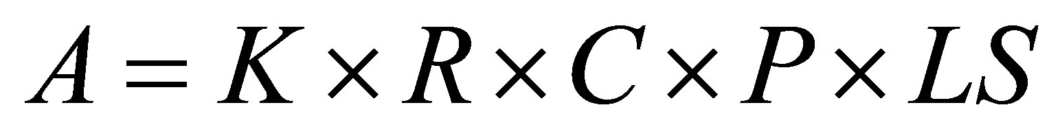 (1)
(1)
whereA = Average annual soil loss per unit area;
K = Soil erodibility factor;
R = Rainfall and runoff erodibility index;
C = Crop/vegetation and management factor;
P = support practice factor;
LS = slope length-gradient factor.
In previous studies, the parameters of soil erodibility factor (K), rainfall and runoff erodibility index (R), and slope length-gradient factor (LS) are extensively studied, for instances Meester and Jungerius (1978), Loch and Rosewell, (1992), had investigated on K factor [4,5], Yu (1999), Mitasova (2002), Ryan (2012) and Mcusburger et al. (2012) had explored on R factor [6-9] and LS factor was studied byJose and Martin (2010) and Liu et al. (2011) [10,11].
However, two other parameters named ascrop/vegetation and management factor (C) and support practice factor (P), are not fully studied yet. Due to the rising awareness of riparian conservation, it is the initiation of this paper to explore on vegetative cover and its conservation or support practice factors to trap the sediment. This study employs Buffer Zone Calculator as a tool to determine the sediment removal efficiency for different C and P.
2. Buffer Zone Calculator
Buffer zone calculator was built up from a series of formulas. Basically, the formulas can be divided into two parts, the determination of buffer width and the outcome assessment of percentage of sediment reduction.
2.1. Determination of Buffer Width
Determination of buffer width is calculated using three following equations:
1) Soil loss or sediment produced on site, calculated by Universal Soil Loss Equation (USLE) [12] as presented in Equation (1).
2) Annual Average total solid concentration is the concentration of sediment flows into the river, calculated using Equation (2).
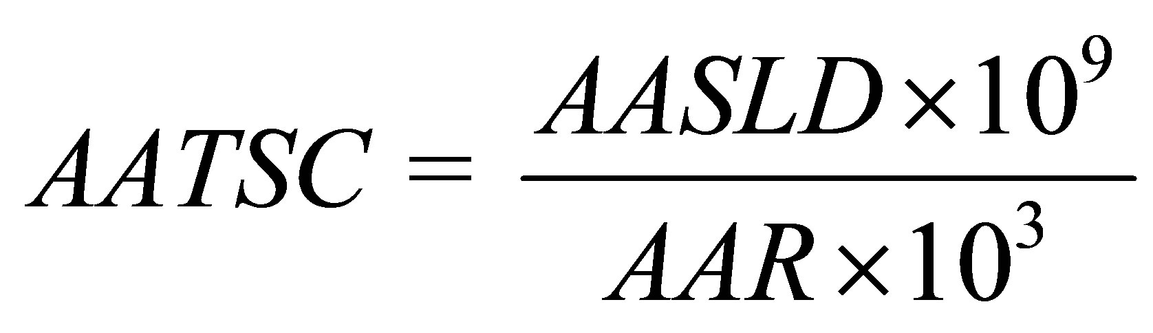 (2)
(2)
where AATSC = Annual Average Total Solid Concentration;
AASLD = Average Annual Solid Loss from Development;
AAR = Average Annual Runoff;
 (3)
(3)
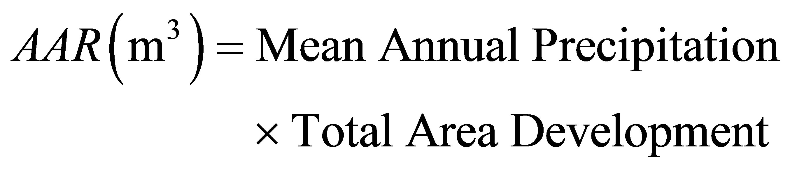 (4)
(4)
3) The required buffer width takes into account the factor of slope [2] and the equation is:
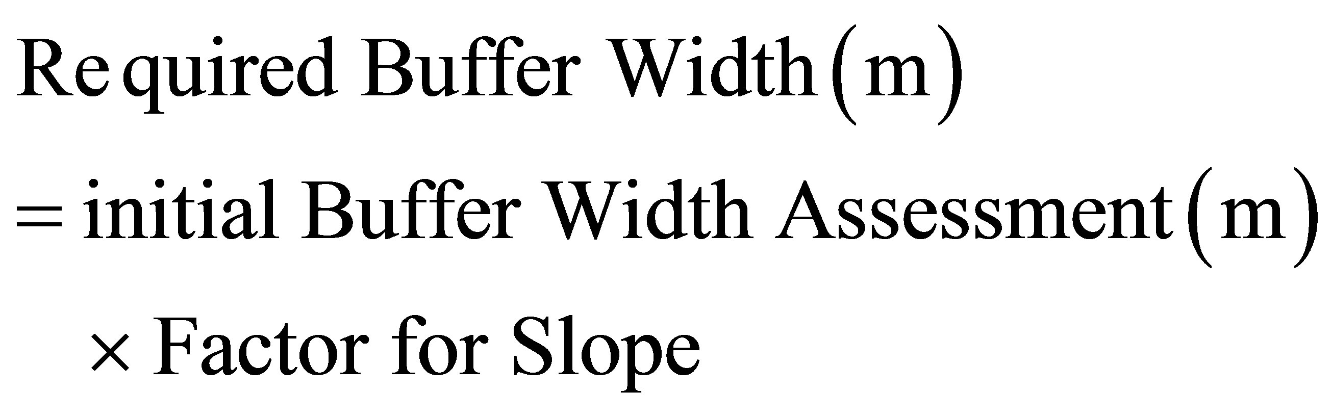 (5)
(5)
2.2. Outcome Assessment
The outcome assessment including Total Suspended Solid (TSS) retained, Outfall TSS and percentage of sediment reduction, are calculated using following equations.
1) Sediment retained by buffer is a function of concentration of TSS retained by vegetation divided by slope of buffer as presented in Equation (6). When the slope is steep, water flows at higher speed through the buffer. Thus, it required wider vegetative buffer width and acquired more time to slowdown the water flow for vegetation in buffer zone to trap sediment [13].
 (6)
(6)
where CRBV = Concentration Retained by Buffer Vegetation (mg/l);
RRBW = Required Riparian Buffer Width (m);
2) Sediment released from buffer is the difference between TSS concentration inflow and TSS retained by buffer, as presented in Equation (7).
 (7)
(7)
where AATSSC = Annual Average TSS Concentration (mg/l);
TSSR = TSS Retained (mg/l).
3) Percentage of sediment reduction is the removal rate of the sediment concentration in the buffer zone [14], as represented in Equations (8) and (9) respectively.
 (8)
(8)
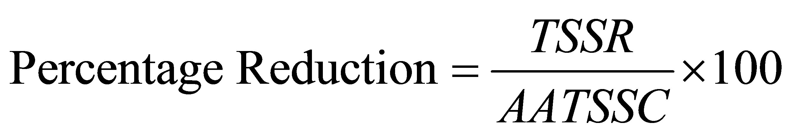 (9)
(9)
3. Study Area
The chosen study area is located at Santubong, which is well known for its fascinating wildlife in Sarawak. As Santubong river flows into South China Sea, Irrawaddy dolph in is always spotted at Santubong river mouth. Along Santubong river, rare proboscis monkeys are always spotted within the mangrove swamps. During night fall, fireflies are flying around the branches of the mangroves and crocodiles are often seen on the mud banks.
Santubong area is categorized as rural catchment. The riparian buffer zone along the Santubong river is presented in Figure 1. The red lines indicate part of the horizontal alignment of Santubong river and Santubong Bridge is circled in yellow.
A site investigation was carried out at the early stage of this study. It was found that the length of buffer zone is about 2500 m and the hill slope length is approximately 200 - 250 m. This area currently is covered by forest, and it is expected to turn into agricultural hub in nearest future. For both sides of Santubong river, it was covered with the buffer zone with the average width of 50 m each site. Both hill slope and buffer gradients are averagely 5%.
4. Methodology
USLE consists of five major factors namely R, K, LS, C and P for calculating the soil loss. In recent years, the parameters of K, R, and LS are extensively studied. However, parameters of C and P are not fully studied yet. Therefore, there is an urgent need to explore and investigate the impact of P and C factors to trap the sediment. In this study, the impact of C and P factors are investigated using Buffer Zone Calculator.
Factor C is used to determine the relative effectiveness of soil and crop management systems in term of preventing soil loss. C factor is a ratio comparing the soil loss from land under a specific crop and management system to the corresponding loss from continuously fallow and tilled land. The C Factor can be determined by selecting the crop type and tillage method that corresponds to the field and then multiplying these factors together. This generalized C factor provides relative numbers for different cropping and tillage systems. Thereby it is able to weigh the merits of each system.
There are 17 alternatives of future land uses available in Buffer Zone Calculator. These 17 different future land uses are forest with undergrowth, forest with no undergrowth, logging 10^6, logging 20, logging 30, mixed dipt. forest, new shifting agriculture, old shifting agriculture, settlement/cleared land, cultivated grass, oil palm plantation, rubber plantation, beans plantation, cocoa plantation, coffee plantation, tea plantation and paddy plantation. The C values for different types of crop investigated are presented in Table 1.
For investigating the impact of C values to the outfall and % reduction of TSS, the selection of C values for different land uses in Buffer Zone Calculator is changing, while 9 other parameters obtained from site investigation are remained constant. The values for these 9 parameters are:
1) soil types = Rjn − Rajang;
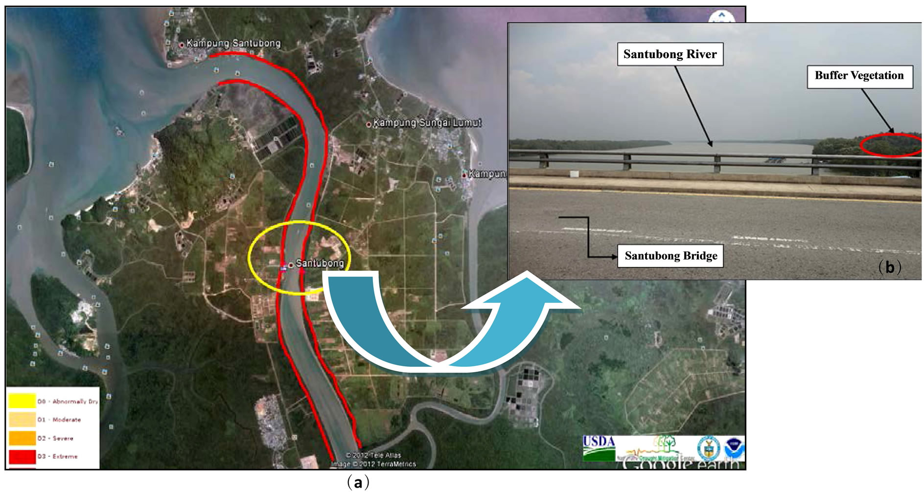
Figure 1. Santubong River with buffer vegetation grown alongside the river. (a) Plan view of Santubong area; (b) View of Santubong river from bridge.
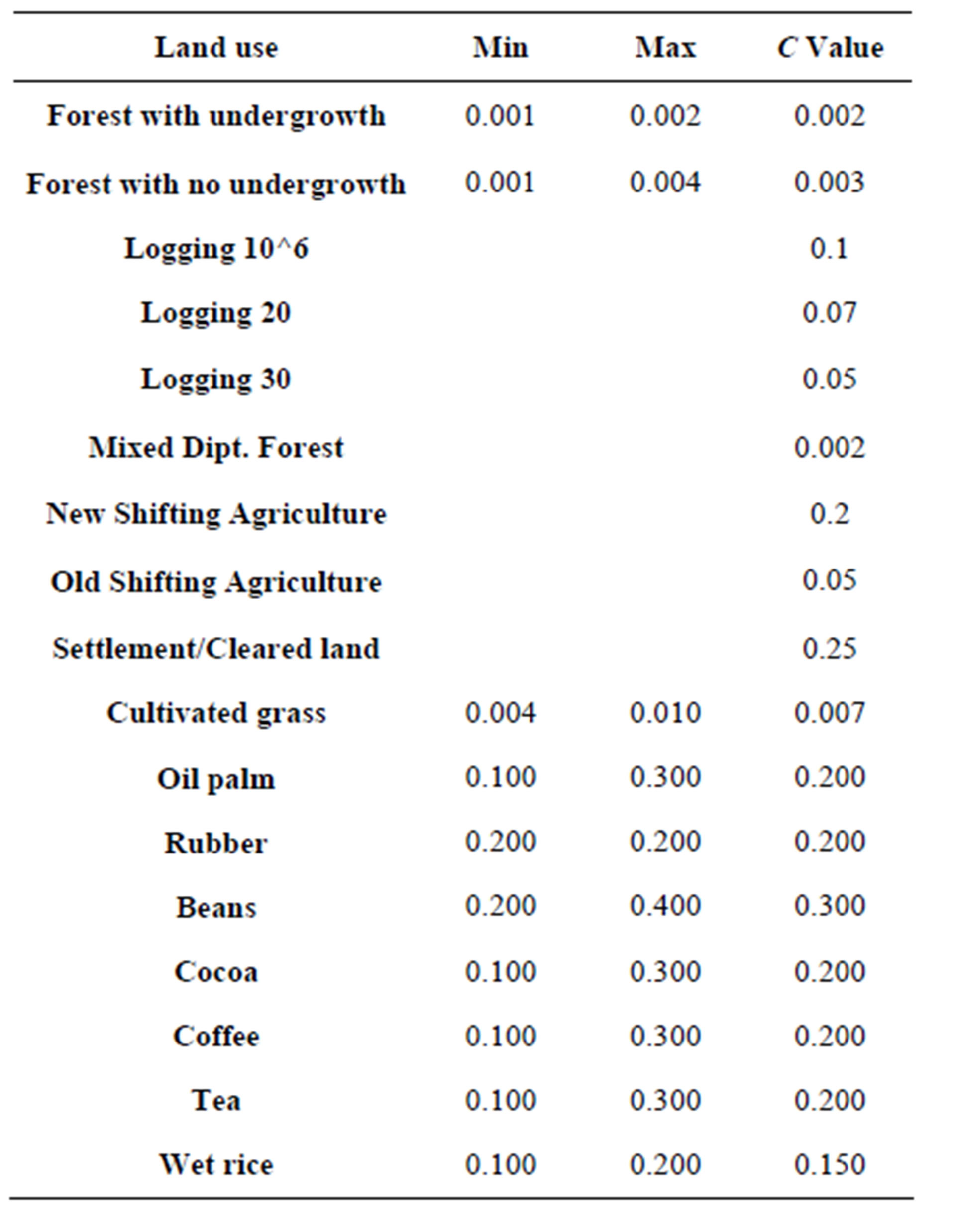
Table 1. C values for different types of crop investigated.
2) mean annual precipitation = 3000 mm;
3) length of hill slope = 215 m;
4) length of buffer = 2300 m;
5) types of buffer vegetation = Forest;
6) gradient of hill slope = 7.5%;
7) gradient of buffer future soil conservation practices = 5%;
8) buffer zone width = 50 m;
9) Soil support practice = none.
Meanwhile, P factor is the support practice factor. It reflects the effects of practices that will reduce the amount and rate of the water runoff and thus reduce the amount of erosion. The P factor represents the ratio of soil loss by a support practice to that of straight-row farming up and down the slope. The most commonly used supporting cropland practices are cross slope cultivation, contour farming and strip cropping.
Table 2 presents P values for different investigated support practice factors. The conservation and support practices available in Buffer Zone Calculator comprised of none, contouring, contouring strip-cropping and terracing. The “none” means that the existing buffer zone at the study area will not undergo any future development and conservation practice. The impact of P factor to the sediment trapping capacity of buffer zone was conducted by selecting one of the practices, while the other 9 factors are remained constant as listed below.
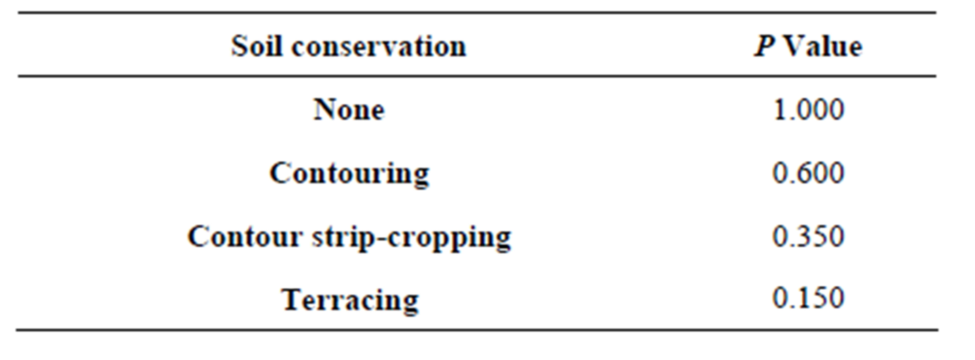
Table 2. P values for different support practice factors.
1) soil types = Rjn − Rajang;
2) mean annual precipitation = 3,000 mm;
3) length of hill slope = 215 m;
4) length of buffer = 2,300 m;
5) types of buffer vegetation = Forest;
6) gradient of hill slope = 7.5%;
7) gradient of buffer future soil conservation practices = 5%;
8) buffer zone width = 50 m;
9) Future land use = Old Shifting Agriculture.
5. Results and Discussion
Table 3 and Figure 2 present the outfall TSS and % reduction of TSS for different future land uses. Basically, different future land uses will produce varies outfall TSS and % reduction of TSS. The predicted outfall TSS for different future land uses are ranging from −161 mg/L to 7571 mg/L, and predicted % reduction of TSS are ranging from 3% to 514%. Negative values obtained for outfall TSS especially from cultivated grass, forest with no undergrowth, mixed dipt. forest and forest with undergrowth, indicate that the buffer is able to reduce the TSS effectively and efficiently until there is no outfall TSS produced in the study area.
From Table 3, it was found that with C value of 0.3 for Beans, the outfall TSS is 7571 mg/l and achieves only 3% of TSS reduction. In contrast, as the C value is 0, the outfall TSS is 0 mg/l and the % reduction of TSS may yield up to 514% especially for forest with undergrowth land use. This indicates that as the C values increase, the outfall TSS is increasing too. At the same time, % reduction of TSS is decreasing. In contrast, C factor of 0 is able to trap the sediment more effective and efficient. Thus resulting high percentage reduction of TSS and low outfall of TSS.
This is because land use with low C factor is able to slow down the flow, assists the filtering process in buffer zone, enhance infiltration and sedimentation activities. Hence, outfall TSS will be reduced effectively. In contrast, an increase of C factor will lead to a decrease in protection by the buffer zone which will eventually increase the soil erosion rate [4].
The effectiveness and efficiency of different soil support practices in reducing TSS are varies. Support practice factor or P factor is the relation between soil loss on
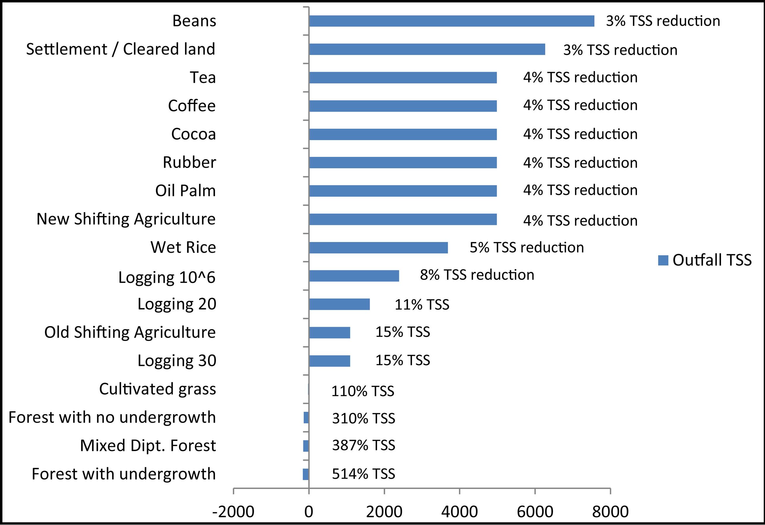
Figure 2. Results of outfall TSS for different future land uses.
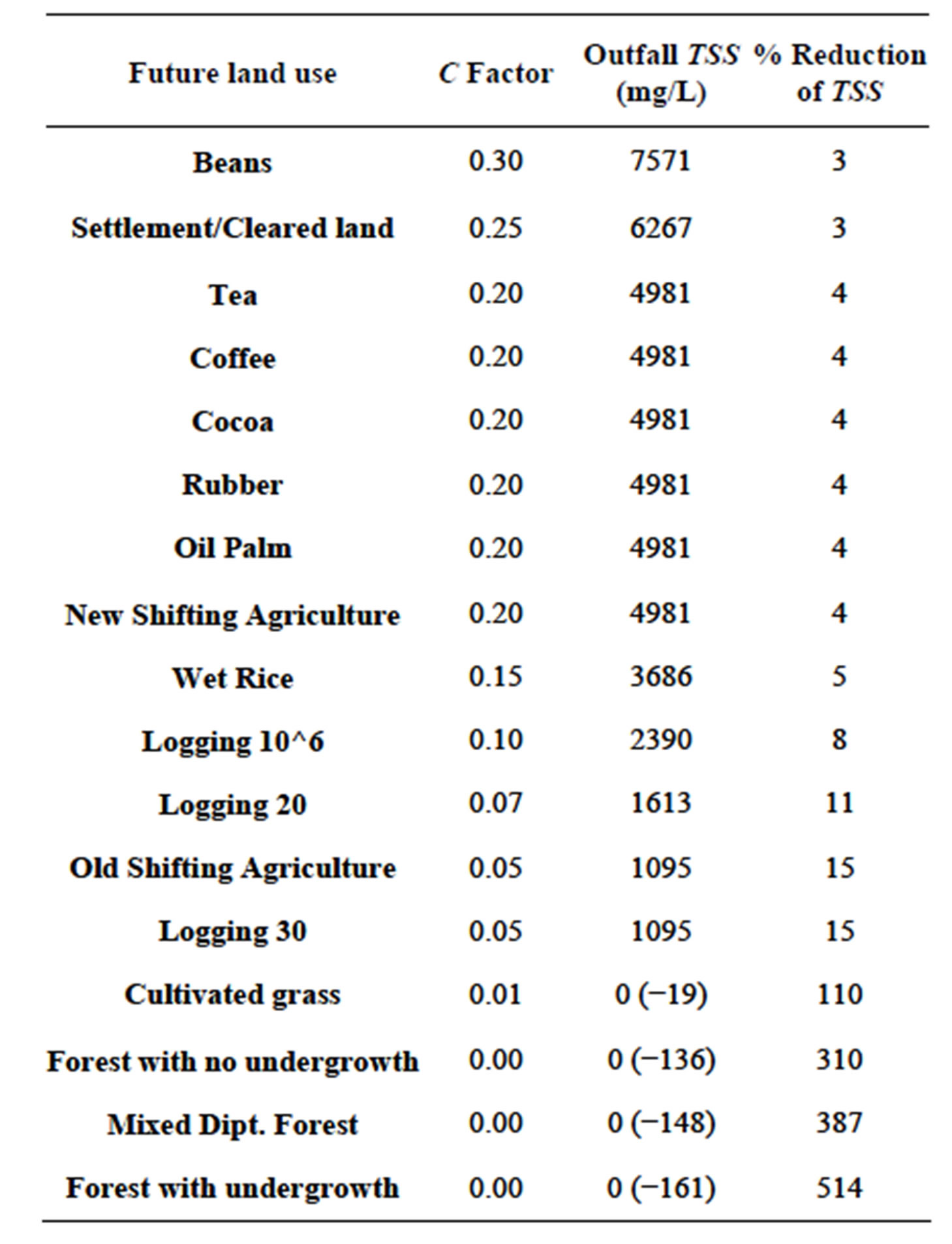
Table 3. Results for outfall and % reduction of TSS with different C values.
a treated field and the topographical factor. Referring to Table 4" target="_self"> Table 4 and Figure 3, the amount of outfall TSS for the no soil conservation practice is 922 mg/L and achieves only 30% reduction of TSS. As the soil conservation practices changed to contouring, contouring strip-cropping and terracing form, the outfall TSS will significantly reduce to 393 mg/L, 63 mg/L and −202 mg/L respectively, and % reduction of TSS will increase to 50%, 86% and 202% respectively. These indicate that the outfall TSS is reducing with the decreasing of P values. Concurrently, the % reduction of TSS will be increased with the decreasing of P values (refer to Table 4).
Results show that the most effective and efficient support practice to reduce the outfall TSS is terracing with P factor of 0.15, followed by contour-strip cropping with P factor of 0.30, and lastly contouring with P factor of 0.60. These support practices are able to reduce outfall TSS efficiently by slowing down the surface runoff.
Contouring is able to reduce the speed of surface runoff due to its different height of land. This provides sufficient time for the surface water to infiltrate and thus reducing the outfall TSS. Meanwhile, contouring also can reduce soil erosion. Besides, contour strip-cropping consists of vegetation plantation along the contour. The vegetation will slow down the surface runoff, trap and filter the sediment more effectively compare to contouring. Meanwhile, terracing usually serve as small dams to alter the water and guide it to the out let as water flow down the terrace. Some terraces are planted with vegetation as well in order to decrease the flow rate of surface runoff. Therefore, it is able to reduce the outfall of TSS efficiently.
6. Conclusions
The impacts of C and P factors affecting the performance of buffer zone have been successfully conducted in this study. It was found that the effectiveness and efficiency of different land uses (C values) and support practices (P
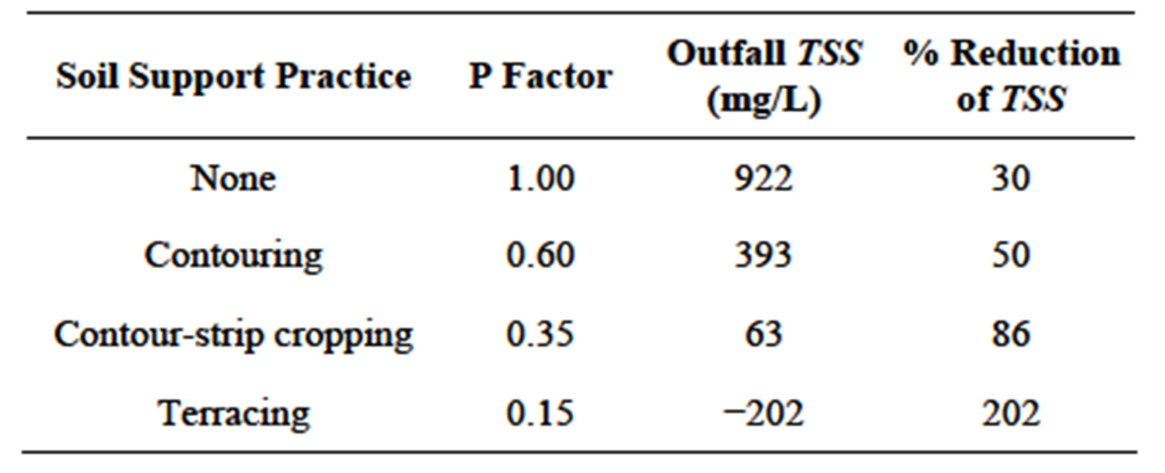
Table 4. Results for outfall and % reduction of TSS with different P values.
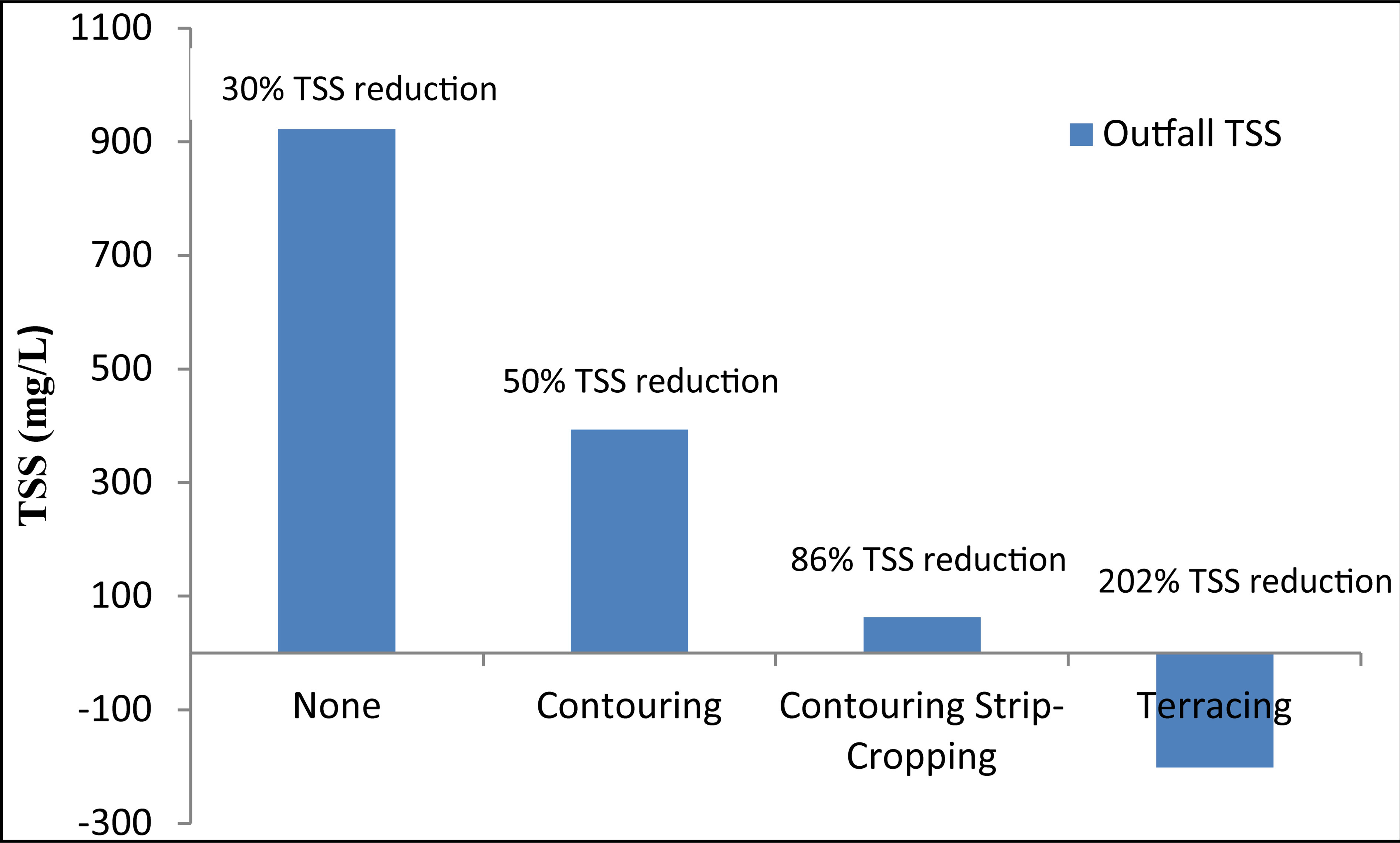
Figure 3. Results of outfall TSS for different future soil conservation practises.
values) soil support practices in reducing TSS are varies. Results show that as the C values increase, the outfall TSS is increasing too, but % reduction of TSS is reducing. Among 17 different land uses investigated, the most effective and efficient land use to reduce TSS in buffer zone is forest with undergrowth, followed by mixed dipt. forest, forest with no undergrowth, cultivated grass, logging 30, logging 10, wet rice, new shifting agriculture, oil palm, rubber, cocoa, coffee, tea and lastly settlement/ cleared land.
Meanwhile, it was found that the % reduction of TSS is increasing with the decrease of P factor. The most effective support practice to reduce the outfall TSS is terracing, followed by contour-strip cropping, contouring and lastly not implementing any soil conservation practice.
REFERENCES
- S. L. Liu, B. S. Cui, S. K. Dong, Z. F. Yang, M. Yang and K. Holt, “Evaluating the Influence of Road Networks on Landscape and Regional Ecological Risk—A Case Study in Lancang River Valley of Southwest China,” Eco Engineering, Vol. 34, No. 2, 2008, pp. 91-99. http://dx.doi.org/10.1016/j.ecoleng.2008.07.006
- K. Arora, S. K. Mickelson and J. L. Baker, “Effectiveness of Vegetated Buffer Strips in Reducing Pesticide Transport in Simulated Runoff,” Transactions of the American Philosophical Society, Vol. 46, 2003, pp. 635-644.
- L. Patty, B. Real and J. J. Gril, “The Use of Grassed Buffer Strips to Remove Pesticides, Nitrate and Soluble Phosphorus Compounds from Runoff Water,” Pesticide Science, Vol. 49, 1997, pp. 243-251. http://dx.doi.org/10.1002/(SICI)1096-9063(199703)49:3<243::AID-PS510>3.0.CO;2-8
- T. D. Meester and P. D. Jungerius, “The Relationship between the Soil Erodibility Factor K (Universal Soil Loss Equation), Aggregate Stability and Micromorphological Properties of Soils in the Hornos Area, S. Spain,” Earth Surface Processes, Wiley, Vol. 3, No. 4, 1978, pp. 379- 391. http://dx.doi.org/10.1002/esp.3290030406
- R. J. Loch and C. J. Rosewell, “Laboratory Methods for Measurement of Soil Erodibilities (K-Factors) for the Universal Soil Loss Equation,” Australian Journal of Soil Research, Vol. 30, No. 2, 1992, pp. 233-248. http://dx.doi.org/10.1071/SR9920233
- B. Yu, “A Comparison of the R-Factor in the Universal Soil Loss Equation and Revised Universal Soil Loss Equation,” ASAE, Vol. 42, No. 6, 1999, pp. 1615-1620. http://dx.doi.org/10.13031/2013.13327
- H. Mitasova, “Geographic Modeling Systems Lab UIUC, Deriving Erosion Modelling Inputs from a Land Cover,” 2012. http://skagit.meas.ncsu.edu/~helena/gmslab/reports/CerlErosionTutorial/denix/Data/deriving_erosion_modeling_inputs.htm>
- L. A. Ryan, “Rainfall Erosivity Attributes on Central and Western Mauritius,” Master of Science (Geography) Thesis, Department of Geography, Geoinformatics and Meteorology, Faculty of Naturaland Agricultural Sciences, University of Pretoria, 2012.
- K. Mcusburger, A. Steel, P. Panagos, L. Montanarella and C. Alewell, “Spatial and Temporal Variability of Rainfall Erosivity Factor for Switzerland,” Hydrology and Earth System Sciences, Vol. 16, 2012, pp. 167-177. http://dx.doi.org/10.5194/hess-16-167-2012
- L. G. R. Jose and C. G. S. Martin, “Historical Review of Topographical Factor, LS, of Water Erosion Models,” Journal of the International Hydrological Programme for Latin America and the Caribbean, Aqua-LAC, Vol. 2, No. 2, 2010, pp. 56-61.
- H. H. Liu, K. Jens, H. Georg and F. Nicola, “Effects of DEM Horizontal Resolution and Methods on Calculating the Slope Length Factor in Gently Rolling Landscapes,” CATENA, Elsevier, Vol. 87, No. 3, 2011, pp. 368-375.
- D. D. Smith, W. H. Wischmeier and Water Conservation Research Division, “Predicting Rainfall-Erosion Losses from Cropland East of the Rocky Mountains: Guide for Selection of Practices for Soil and Water Conservation,” US Department of Agricultural, 1965.
- E. D. Masanja, “Effectiveness of Selected Vegetation Cover Types as Sediment Filters: A Case Study of Lake Victoria Shore Line, Magu District, Tanzania,” Sokoine University of Agricultural, Morogoro, Tanzania, 2009.
- N. Syversen, “Effect and Design of Buffer Zones in the Nordic Climate: The Influence of Width, Amount of Surface Runoff, Seasonal Variation and Vegetation Type on Retention Efficiency for Nutrient and Particle Runoff,” Ecological Engineering, Vol. 24, 2005, pp. 483-490. http://dx.doi.org/10.1016/j.ecoleng.2005.01.016
NOTES
*Corresponding author.