Journal of Water Resource and Protection
Vol.4 No.11(2012), Article ID:24430,15 pages DOI:10.4236/jwarp.2012.411109
Bayesian Data Fusion (BDF) of Monitoring Data with a Statistical Groundwater Contamination Model to Map Groundwater Quality at the Regional Scale
Earth and Life Institute, Université Catholique de Louvain, Louvain-la-Neuve, Belgium
Email: marnik.vanclooster@uclouvain.be
Received August 3, 2012; revised September 9, 2012; accepted October 13, 2012
Keywords: Groundwater Pollution; Nitrate; Kriging; Regression Tree; Data Fusion; Brusselian Sands
ABSTRACT
Groundwater contamination by nitrate within an unconfined sandy aquifer was mapped using a Bayesian Data Fusion (BDF) framework. Groundwater monitoring data was therefore combined with a statistical groundwater contamination model. In a first step, nitrate concentrations, measured at 99 monitoring stations irregularly distributed within the study area, were spatialized using ordinary kriging. Secondly, a statistical regression tree model of nitrate contamination in groundwater was constructed using land use, depth to the water table, altitude and slope as predictor variables. This allowed the construction of a regression tree based contamination map. In a third step, BDF was used to combine optimally the kriged nitrate contamination map with the regression tree based model into one single map, thereby weighing the kriged and regression tree based contamination maps in terms of their estimation uncertainty. It is shown that BDF allows integrating different sources of information about contamination in a final map, allowing quantifying the expected value and variance of the nitrate contamination estimation. It is also shown that the uncertainty in the final map is smaller than the uncertainty from the kriged or regression tree based contamination map.
1. Introduction
Assessing the quality of groundwater is a prerequisite for designing sustainable water management strategies e.g. when implementing the Water Framework Directive [1]. Groundwater quality is, however, a spatially distributed attribute. It is generally accepted that knowledge of the spatial distribution of this attribute allows the design of site specific protection and remediation measures. Therefore robust and validated techniques are needed to map the spatial distribution of groundwater quality within the groundwater body continuum. Unfortunately, properties related to groundwater quality, such as nitrate concentration, can only directly be measured at the local scale. The mapping of groundwater quality within the water body continuum will therefore often build on data interpolation or prediction of properties related to groundwater quality through deterministic or stochastic models, and the adopted technique will impact the results of the final assessment.
Point data can be spatialized with traditional interpolation tools such as Voronoi tessellation, inverse distance weighting or kriging. References [2,3] for instance used ordinary kriging for mapping the spatial variability of nitrate concentrations in a shallow water body. Reference
[4] used Gaussian simulation techniques to introduce local uncertainty for mapping nitrate concentrations within the groundwater bodies of the Po Valley (Italy). Among modern interpolation techniques, the Bayesian Maximum Entropy (BME) framework was developed recently by [5] as a generalization of classical techniques. Reference [6] used BME as a formal spatial modeling framework allowing introducing the temporal variability of groundwater contamination and the sampling rate in a spatial map.
Unfortunately, the locations where groundwater quality properties are measured are typically scarce and sparsely distributed over space. As a result, large uncertainties about the variable of interest arise in the mapping process, especially at prediction points located far away from monitoring stations. Given that the quality of the interpolation decreases rapidly with the distance to the monitoring station, the mapping of a variable of interest through classical geostatistical interpolation techniques will have limited practical utility in regions where a densely distributed monitoring network is not available. Unfortunately, this is rather the rule than the exception, and therefore alternative robust and validated methods are needed to provide more comprehensive and accurate information about the groundwater quality. Data fusion is such a method that can be used to combine optimally various sources of information about groundwater quality in a consistent and accurate model prediction.
Data fusion techniques have already been used in various application fields, including for example biometrics verification systems (e.g. [7,8]), surveillance systems (e.g. [9]), robotics (e.g. [10]), medical imagery (e.g. [11]) or military/civil engineering (e.g. [12,13]). Data fusion has also important applications in classification of remote sensing images (e.g. [14]) and in environmental modeling [15].
Among different data fusion techniques, a Bayesian Data Fusion (BDF) approach was recently proposed by [15]. It was especially designed for spatial predictions problems and provides a consistent framework of fusing an arbitrary large number of information sources that are related to a same variable of interest in order to provide a unique spatial prediction. The main advantage of a Bayesian approach is to put the problem of data fusion into a clear probabilistic framework. Since this original paper, the general method has been applied to various case studies of environmental sciences; remote sensing [16, 17], hydrology [18,19] or air pollution [20]. Similarly to these applications, the present paper relies on some specific assumptions with the aim of spatial mapping of groundwater quality. To the best of our knowledge, BDF has never been used for mapping groundwater pollution by nitrate.
In this paper, we used the BDF approach as a formal framework to map groundwater contamination by nitrates. Groundwater contamination by nitrate remains a critical water quality issue for many groundwater bodies all over the world. The approach was illustrated for mapping groundwater contamination in the water body of the Brusselian sands located in an unconfined sandy aquifer in the centre of Belgium. This water body is considerably affected by nitrate pollution.
Groundwater nitrate concentrations were measured at different monitoring stations irregularly distributed in the study area. In a first step, these point data were interpolated on a grid covering the whole study area by a classical (ordinary kriging) geostatistical technique. With this interpolation method, the uncertainty on the prediction depends partly on the respective geometry of the monitoring station and the estimation point. As a consequence, the uncertainty on the predictions is larger in parts of the study area where data are scarce, making these estimates useless at some points on the map. Secondly, nitrate concentrations were predicted by a statistical model all over the study area. With this model, the prediction uncertainty depends on the uncertainty of underlying predictor variables such as depth to the water table, land use or altitude, along with the model uncertainty. In a third step, nitrate concentrations estimated by the interpolation method were combined with those obtained from the statistical model into a single prediction. In this step, BDF is used. The BDF prediction together with its estimated uncertainty was further spatially mapped.
2. Study Area and Data
This study focuses on the unconfined sandy groundwater body located in the Brusselian aquifer in the center part of Belgium. The aquifer has a surface area of 965 km2 and is of primary importance for drinking water supply. This unconfined aquifer is located in Tertiary sands and is overlaid by a Quaternary loess layer of variable thickness (0 to 15 m). The Brusselian sands outcrop mainly in the valleys where sandy and sandy loam soils develop. Transmissivity of the aquifer varies from 2.9 × 10⁻⁵ to 1.2 × 10⁻² m2/s and its permeability varies from 1.4 × 10⁻⁶ to 6 × 10⁻³ m/s [21].
This aquifer is characterized by both the presence of intensive arable cropping and intense urban pressure. The 1:10.000 land use map with 65 land use classes of the Walloon Region was provided by the regional administration and depicts the situation of 2005 [22]. The land use is highly fragmented. Typical land uses are urban (generally located in the valleys; about 17% of land use in the study area), grassland and forests (found on valley slopes; about 13% and 10%, respectively), and arable land, mainly wheat, sugar beet, maize and barley (found on loamy soils on the plateau; about 51% of land use).
The depth to the water table was calculated by subtracting the piezometry value from a 30 m resolution digital elevation model (DEM) which was furnished by the regional administration. The piezometry map was calculated by interpolating the water table levels measured in 1984 using ordinary kriging. The calculation of depth to the water table varies from 0 to more than 45 m with a mean value of 10.5 m.
The groundwater nitrate concentration data used in this study was recently collected over 99 monitoring stations in January and February 2009. These monitoring stations are wells, galleries, drains and springs. A one-way analysis of variance was performed for comparing the nitrate concentrations measured in the different types of monitoring stations and no significant differences were detected in the mean concentrations of the different groups at a significance level of 0.05. The nitrate concentrations show a wide spatial variability in the study area, with values going from 6.9 up to 93.4 mg NO3/L. The regional mean and standard deviation are respectively equal to 45.6 and 17.2 mg NO3/L (Table 1). A Lilliefors test was performed using the function implemented in the Statistics ToolboxTM of MatlabTM. This test confirmed the Gaussian shape of the distribution of the measured nitrate concentrations at a significance level of 0.01.
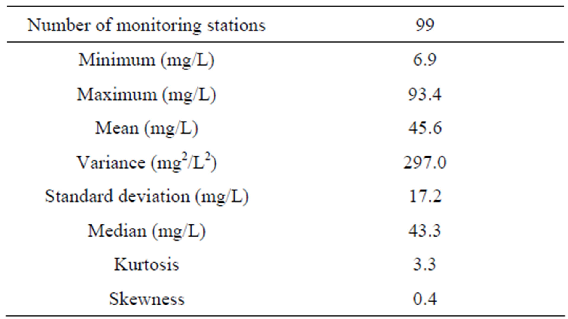
Table 1. Descriptive statistics of the measured nitrate concentrations.
3. Tools and Methods
3.1. Kriging
Kriging is a group of stochastic prediction techniques widely used in geostatistics to interpolate the value of a random field (e.g., the groundwater nitrate concentration) at an unobserved location, based on a linear combination of observed values at nearby locations. Kriging incorporates the spatial dependence of the data in its estimation process through a variogram or a covariance function. The variogram function yields the average dissimilarity between locations separated by different intervals of distances. Kriging is known to provide a linear predictor that corresponds to the Best Linear Unbiased Predictor (BLUP) in the least squares sense. Additionally, it is the best possible predictor when random field is assumed to be multivariate Gaussian. Ordinary kriging is the most commonly used type of kriging. It assumes a constant but unknown mean and enough observations to reliably estimate the variogram.
3.2. Regression Tree
Regression tree modeling is an explanatory technique relying on a process known as binary recursive partitioning. Regression trees became popular in environmental sciences in the early nineties (e.g. [23-25]). The algorithm identifies which of the variables explains most of the variance in the response variable, then determines the threshold value of the explanatory variable that best partitions the variance in the response such that it minimizes the sum of the squared deviations from the mean in the two groups. The process is repeated for each new branch until there is no residual explanatory power, according to the limitations imposed by the user. Suppose that predicttor variables x1, x2, ···, xN and the response variable y are organized as columns in a table. The database table is sorted by the column of the first variable (x1). Then the table is split into two parts (called left and right branch) until the number of samples in the branch to split is lower than a user defined threshold. For each possible split position, the two partitions are compared based on the reduction in non-homogeneity
 (1)
(1)
that they provide. The non-homogeneity in a group of samples is measured by computing deviations and is defined as
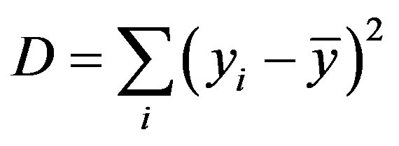 (2)
(2)
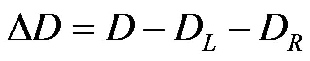
where  is the mean value across all observations yi. Each partition generates left (DL) and right (DR) deviance values. This process is repeated for each of the N predicttor variables. The partition that maximizes the change in deviance ΔD is the partition to choose. Each of the branches obtained after partitioning is partitioned again using the same method.
Regression trees are often used to see whether complex interactions between explanatory variables exists and to identify which one of the predictors have the most important effect on the dependent variable [26]. Major advantages of regression tree models are that 1) they are nonparametric and, hence, Gaussian distribution assumption of predictor variables does not need to be satisfied, 2) they can incorporate categorical data, and 3) they allow possibly complex interactions between the predictor variables to be represented without assumptions of linearity. Furthermore, while multiple linear regression identifies global relationships in the data set, regression tree are able to identify local relationships [27].
In this study, a regression tree was developed for predicting nitrate concentrations as a function of the predicttors listed in Table 2. The regression tree model was
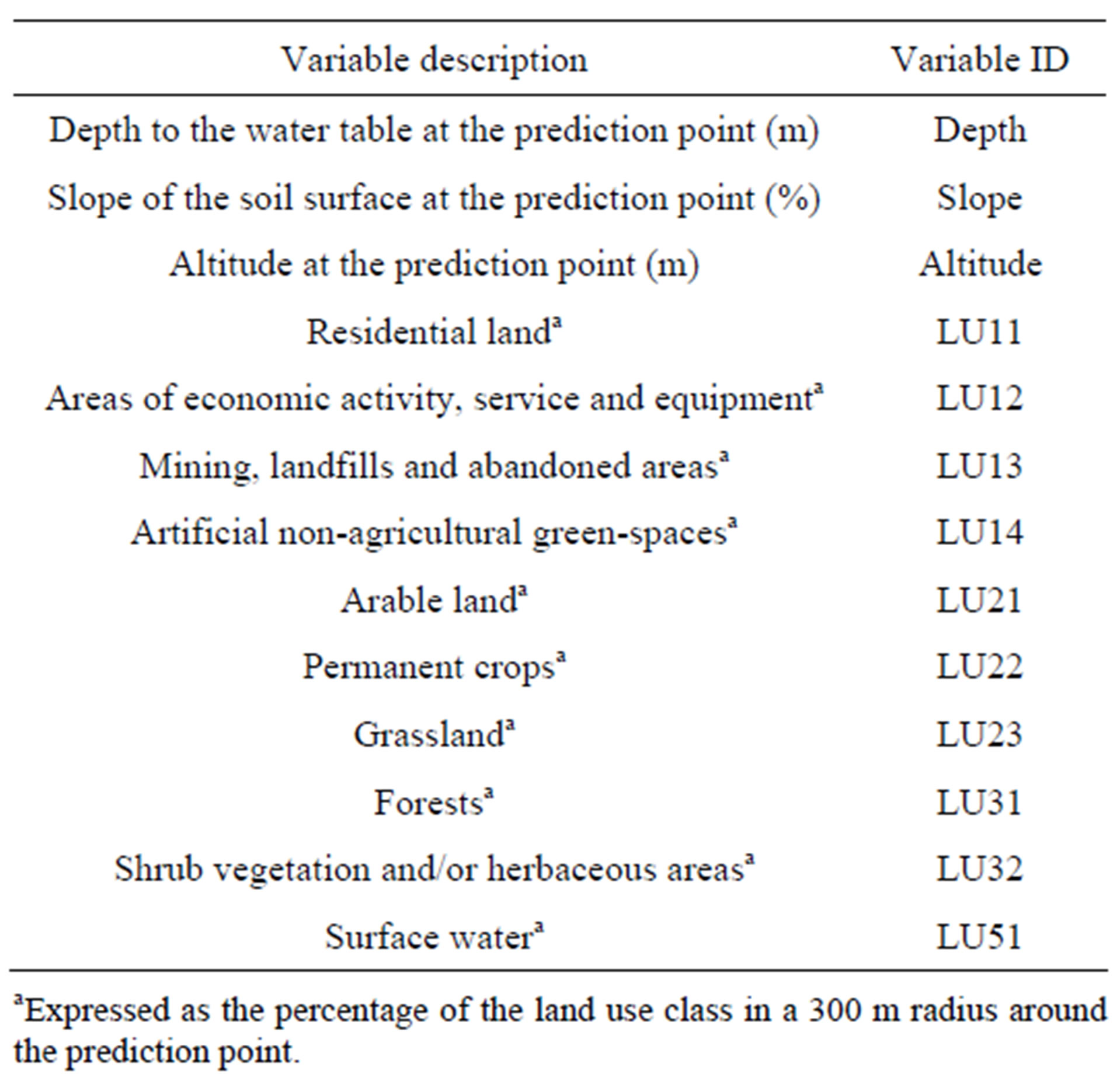
Table 2. Description of the variables used in the regression tree model.
applied to the dataset to predict nitrate concentrations all over the study area at the nodes of a regular 50 m × 50 m grid.
Regression tree algorithms are implemented in various software packages such as MatlabTM, SASTM, R. The “classregtree” function implemented in the Matlab Statistical ToolboxTM was used in this study.
3.3. Bayesian Data Fusion (BDF)
The Bayesian data fusion approach relies on the hypothesis that one can decompose the spatial component (i.e. the prior distribution) from the other information sources (i.e. the likelihood function). Subsequently, one can assume that, conditionally to the true underlying variable, the different information sources are independent. In the Bayesian framework, this implies directly that the likelihood function can be decomposed in a product of conditional distributions. The Bayes’s theorem can thus be applied a second time in order to express the posterior distribution of a given variable Z0 given the other secondary variables Yi either as a function of the conditional distribution  or
or . It is beyond the scope of this paper to present the whole underlying theory of BDF. For more details about the general description of the approach, the reader can consult [15,18] for a specific implementation of the approach.
The general BDF equations can be simplified to simple analytical formulas when it is assumed that the distributions of errors obtained by kriging and by the statistical model are Gaussian [18]. The final predicted mean nitrate concentration μP and its variance  are then given by
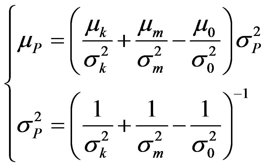 (3)
(3)
where μk, μm and μ0 are the means associated with the kriging prediction, the statistical model prediction and a “rough” estimation of the local mean obtained from the inverse distance method, respectively, and where ,
,  and
and  are the variances associated with the kriging prediction (defined as the variance of prediction Var(Zest,0 – Z0), where Zest,0 is the predicted value and Z0 the observed value), the variance associated with the statistical model prediction (defined as the variance of the data at the end of each branch of the regression tree) and the sill of the semi-variogram, respectively.
3.4. Comparison of Methods
The presented interpolation methods yield different cartographic results because of their inherent characteristics. Each map is subject to prediction errors. To elucidate those errors and to illustrate the estimation accuracy, a “leave-one-out” cross-validation approach was performed. The following indicators were chosen for accuracy assessment:
The root mean squared error (RMSE):
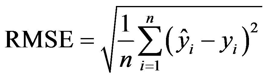 (4)
(4)
The mean absolute error (MAE):
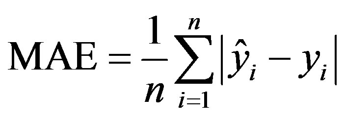 (5)
(5)
The mean error (ME):
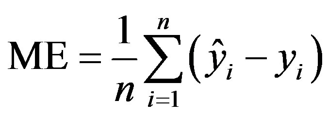 (6)
(6)
The coefficient of determination (R2):
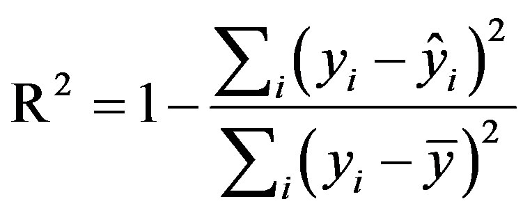 (7)
(7)
where n is the number of observations,  is the mean value across all observations yi and ŷi are the predicted values.
It is worth noting that these quality indicators only reflect the general regional accuracy of the predictions. Local improvements of the mapping process must therefore be observed directly on the maps of uncertainties.
All calculations were performed in MatlabTM R2008b, using the geostatistical BMElib package [5]. Data preparation was carried out in ArcGISTM 9.3.
4. Results
4.1. Kriging
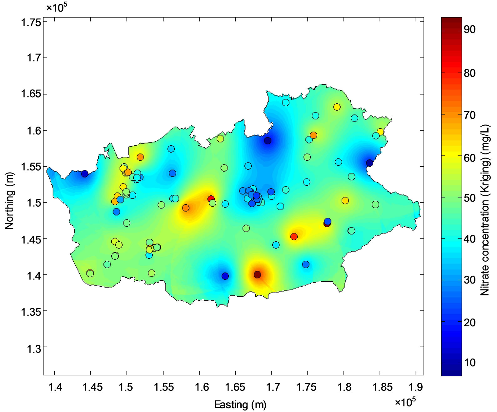
The first presented mapping method relies on the interpolation of the measured nitrate concentrations through ordinary kriging. An experimental semi-variogram was modeled as the sum of a nugget effect of 67.2 mg2/L2 and an exponential model with total theoretical variance and range of 332.9 mg2/L2 and 12090.8 m, respectively (Figure 1). About 66.5% of the study area has kriged nitrate concentrations lower than the standard of 50 mg/L, while nitrate concentrations exceeding 80 mg/L are observed in some parts of the study area (Figure 2(a)). The predicttion errors of the kriged concentration is minimum at the location of the monitoring stations and raises up to 20 mg/L were the density of the monitoring stations is the lowest (Figure 2(b)).
Kriged nitrate concentrations were compared to measured nitrate concentrations by a “leave-one-out” cross validation (Figure 3). The data roughly scatter around the 1:1 line. This bad prediction quality is partly due to
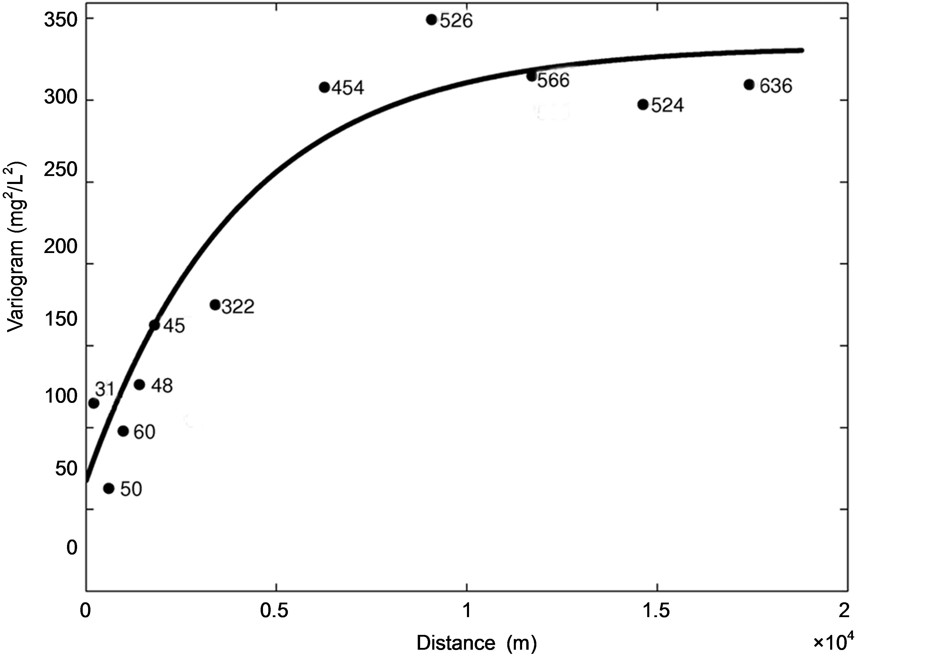
Figure 1. Semi-variogram of the nitrate concentrations in the Brusselian sands estimated on the basis of the dataset of January and February 2009. Dots represent the experimental semi-variogram (together with the number of data pairs on each lag interval), plain line represents the fitted semi-variogram.
 (a)
(a)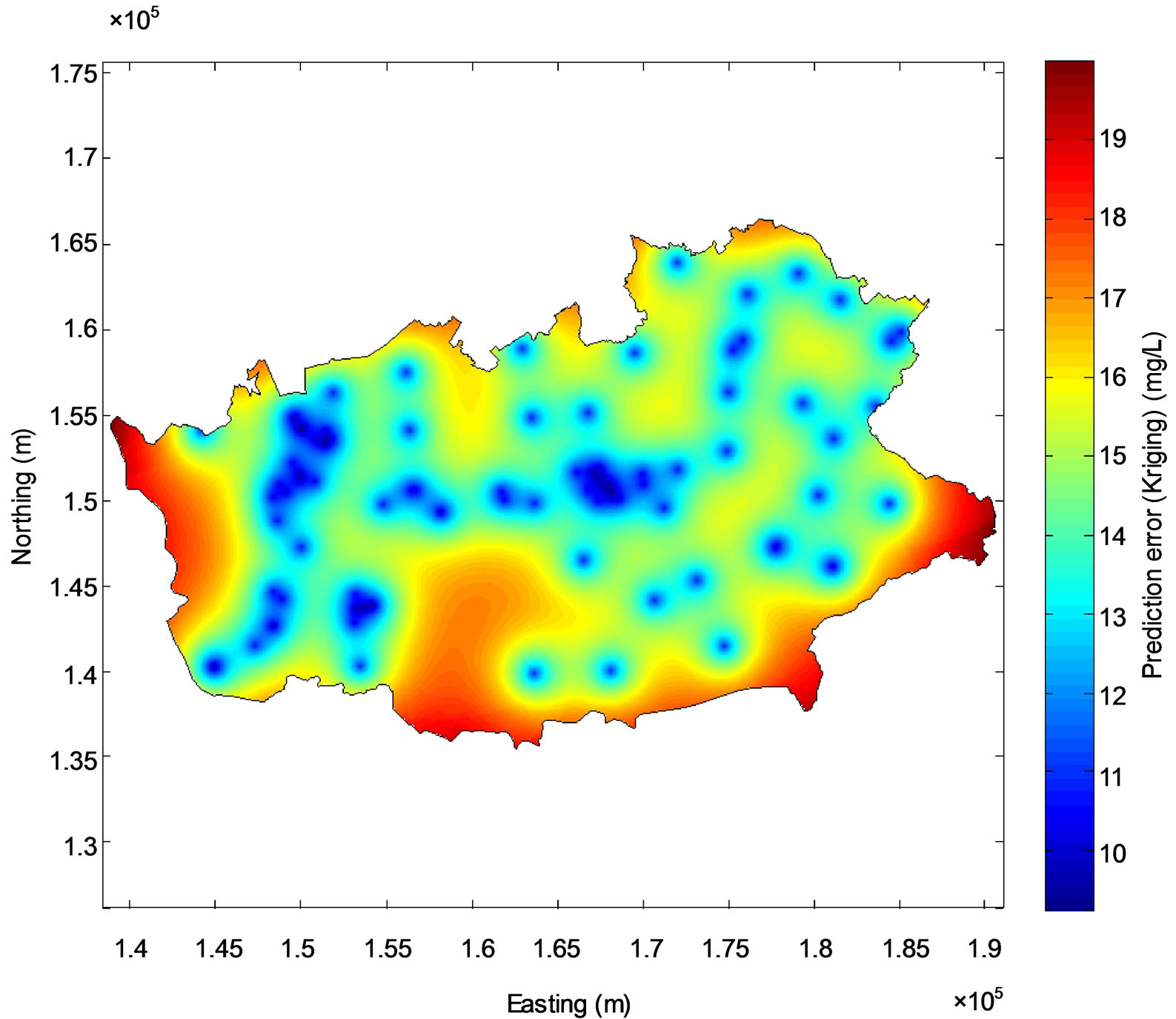 (b)
(b)
Figure 2. Map of kriged groundwater nitrate concentration (a) and associated prediction error (b). The monitoring stations are symbolized by circles on (a).
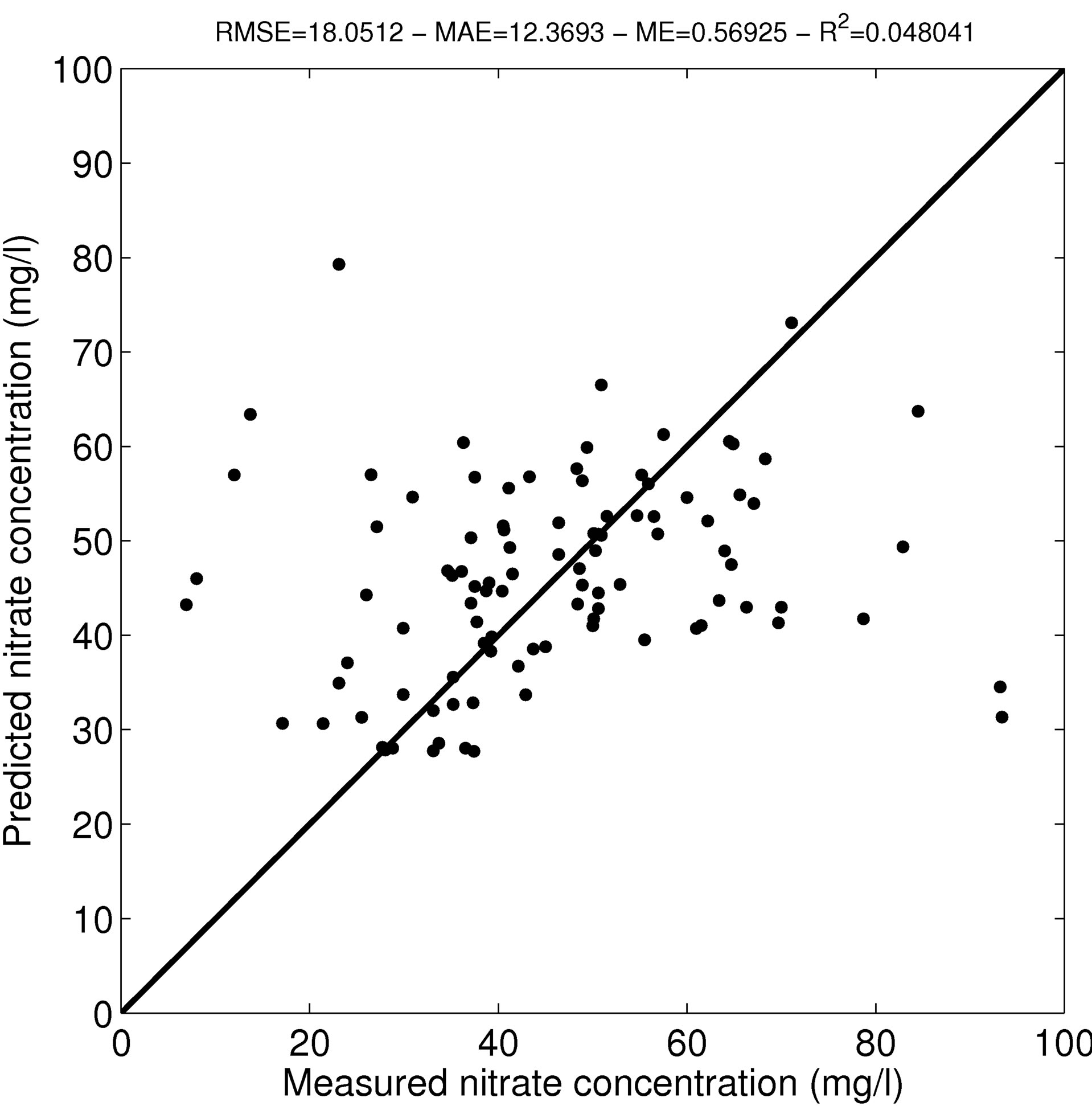
Figure 3. Comparison of the kriged nitrate concentrations to the measured nitrate concentrations. The plain line represents the 1:1 line.
the very low density of the sampling network in some parts of the study area. As a consequence, when the “leave-one-out” cross validation process removes these isolated points from the dataset, the prediction solely relies on data located far away from that point, thus resulting in an inaccurate prediction and a global poor coefficient of determination. Furthermore, the presence of a nugget effect of about 20% of the total variance is also responsible for poor prediction results.
4.2. Regression Tree
4.2.1. Development of the Regression Tree
Nitrate concentrations measured at the 99 monitoring stations in January and February 2009 were related to the 13 variables listed in Table 2 through a regression tree model (Figure 4(b)). As shown by [28] such models show highly complex interaction patterns, suggesting that it is a complex combination of variables that explains ob-served pollution levels, rather than single explicative variables.
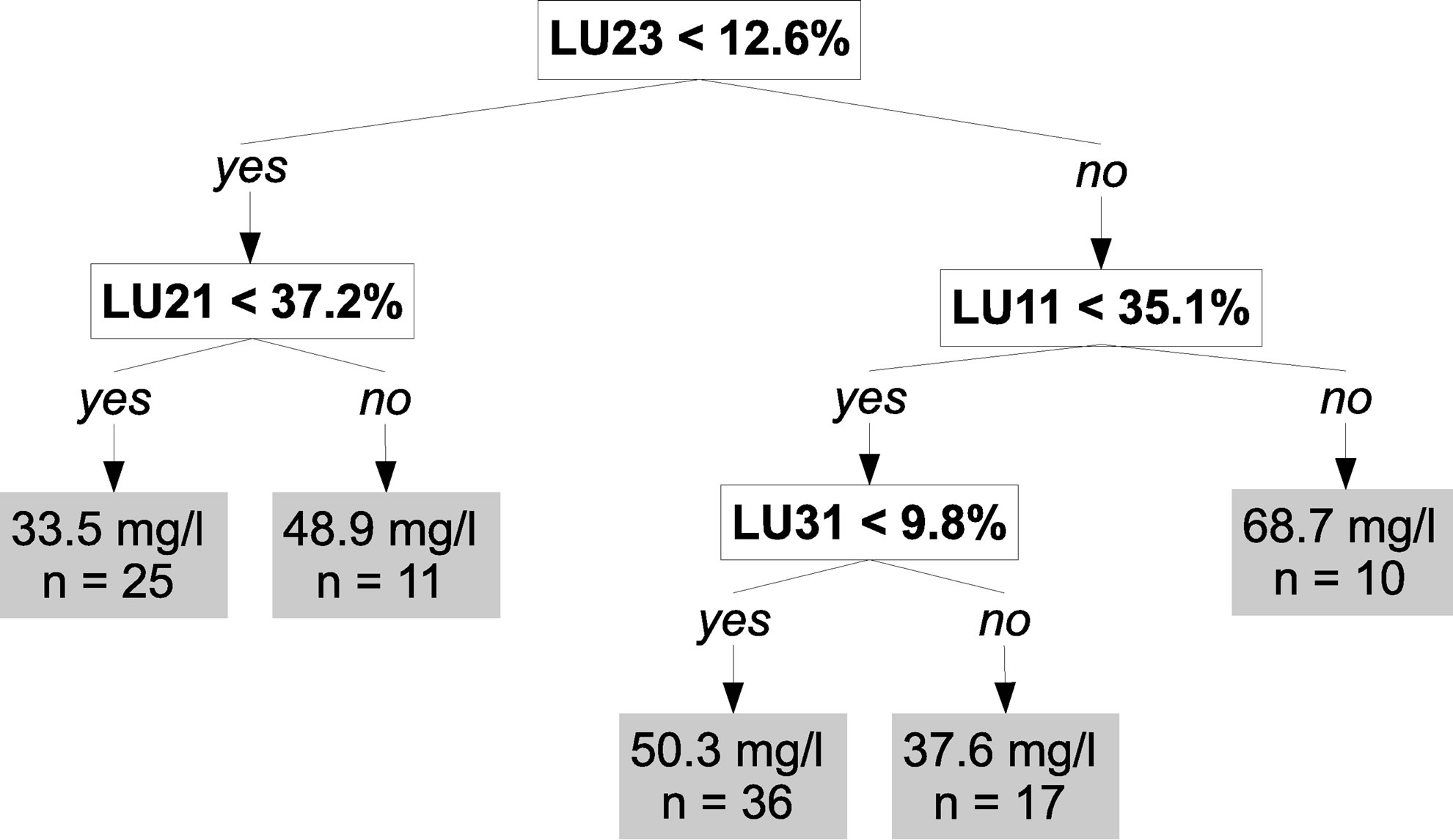
Figure 4(a), which represents a simplified version of the regression tree with only the upper part of the tree,
 (a)
(a)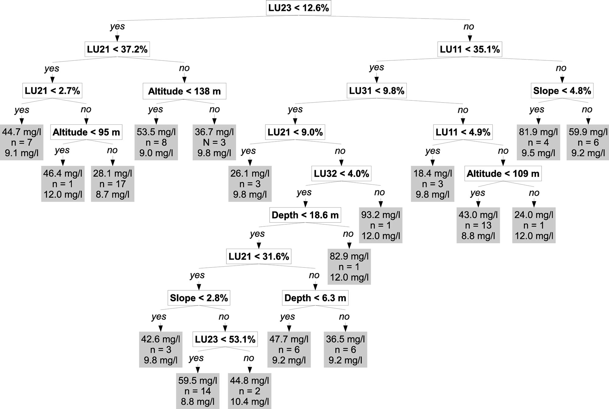 (b)
(b)
Figure 4. Simplified (a) and complete (b) regression trees. At the end of each branch, the first value is the mean nitrate concentration; the second value is the number of samples and the third value is the prediction error. See Table 2 for legend.
shows that the most important explanatory variable is the percentage of grassland in a 300 m radius around the prediction point (LU23) and the threshold value separat-ing low and high values of LU23 is 12.6%. For low val-ues of LU23, the tree shows that the percentage of arable land in a 300 m radius around the prediction point (LU21) has a significant impact on groundwater pollution by nitrate. Indeed, lower mean nitrate concentration (33.5 mg/L) are observed where less than about one third of the area around the prediction point is covered by arable land (LU21 < 37.2%). For high values of LU23, the tree shows that the percentage of residential land in a 300 m radius around the prediction point (LU11) is significant. High values of LU11 (>35.1%) result in high mean nitrate concentration (68.7 mg/L), while for lower values of residential land (LU11 < 35.1%) the mean nitrate concentration is lower and depends also on the percentage of forests in a 300 m radius around the prediction point.
The regression tree was applied to the dataset and the estimated nitrate concentrations were compared to the measured nitrate concentrations resulting in an R2 of 0.80 and an RMSE of 7.66 mg/L (Figure 5). All parameters of the model are significant at the 0.05 level.
4.2.2. Prediction with the Regression Tree
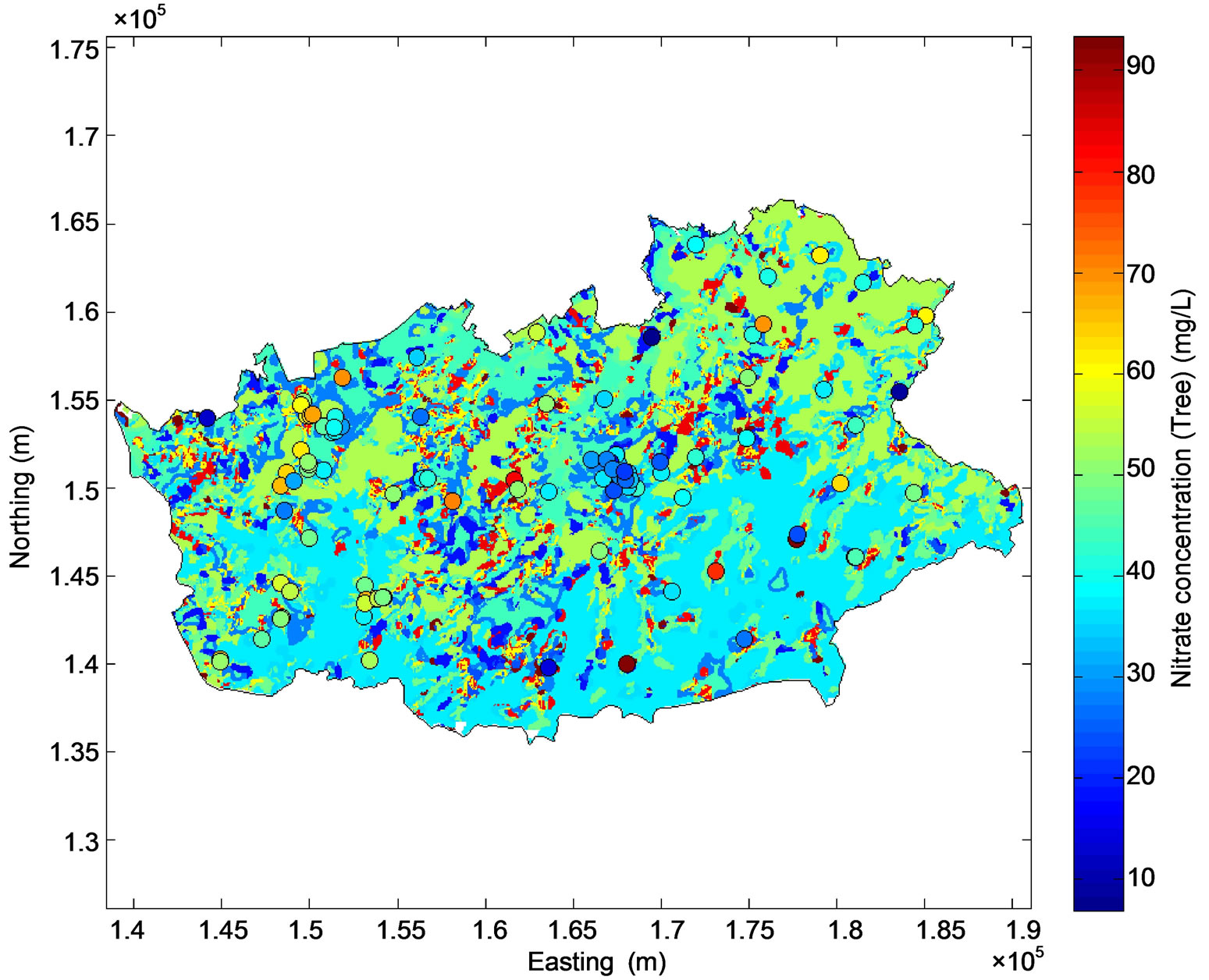
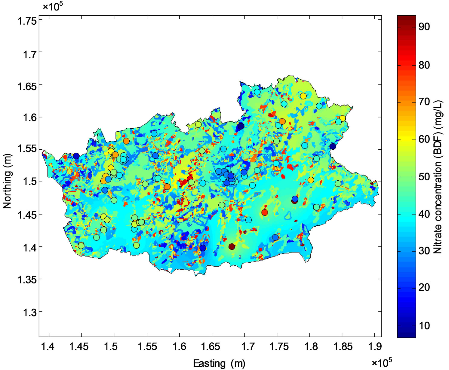
The regression tree model was applied to the gridded dataset using variables listed in Table 2 to predict nitrate concentration at the nodes of the prediction grid. About 70.9% of the study area has predicted nitrate concentrations lower than 50 mg/L (Figure 6(a)). As expected from the regression tree, the highest nitrate concentrations are observed in urban areas of the central and northwest parts of the study area, while lower concentrations are observed in the south-west and south-east. The prediction error of the regression tree model ranges from 9 to 12 mg/L (Figure 6(b)).
4.3. Bayesian Data Fusion (BDF)
The BDF method uses the results of the prediction map provided by the kriging interpolation model and the map resulting from the regression tree model for fusing these two information based on a weighing according their relative prediction errors. The nitrate concentration predicted by kriging will be preferred at places where the kriging prediction error is smaller than the prediction error of the regression tree, and reciprocally. Since the prediction error of the regression tree map is generally lower than for kriging, the BDF map is very close to the map made by the regression tree, except near the monitoring stations. In the map predicted by BDF, 64.6% of
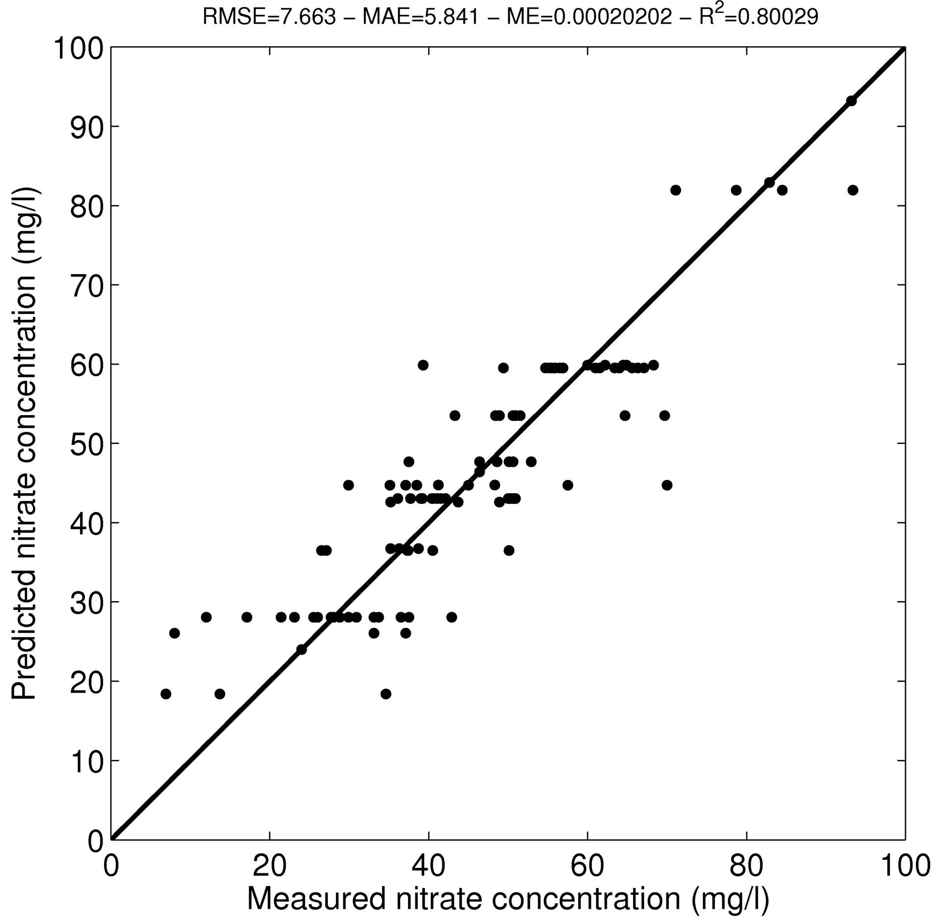
Figure 5. Comparison of the nitrate concentrations predicted with the regression tree model to the measured nitrate concentrations. The plain line represents the 1:1 line.
the study area has predicted nitrate concentrations lower than 50 mg/L (Figure 7(a)) and the prediction error varies from less than 7 to about 12 mg/L (Figure 7(b)). The ni-trate concentrations estimated with BDF were compared to the measured nitrate concentrations resulting in an R2 of 0.74 and an RMSE of 8.77 mg/L (Figure 8).
5. Discussion
Nitrate concentrations measured at 99 monitoring stations irregularly distributed in the study area were spatialized on the whole region by both ordinary kriging interpolation and a statistically based regression tree model. The kriging predictions have the lowest uncertainties at proximity of the monitoring stations and huge uncertainties further away, while the predictions made by the regression tree have more homogeneous uncertainties throughout the study area. Also kriging is an exact predictor, meaning that the concentration predicted at the locations of the measuring points is equal to the measured value, but the regression tree model only predicts an expected value. As a consequence, the measured concentration do not honors the measurements on the map constructed from the regression tree. Using Bayesian Data Fusion allows combining the nitrate concentrations estimated by the interpolation method with those estimated by the statistical model into a single final map and allows us to reduce the associated prediction uncertainty.
The quality of the map constructed from the kriging method is influenced by the density and geometry of the monitoring network. In low density sampling regions, a local pollution could be wrongly extrapolated to a big surrounding area. These singular points (with local extreme concentrations) are responsible for the global poor coefficient of determination resulting from the “leaveone-out” cross validation process. While they could be considered as outliers in a pure kriging process, and therefore removed from the analysis, these points make sense in a BDF framework since they will be weighted with the predictions made by the regression tree model.
The regression tree was able to estimate nitrate concentrations at the unsampled parts of the study area with a lower uncertainty than the kriging method (Figures 2(b) and 6(b)). The fragmented aspect of the map constructed from the regression tree is due to the discontinuous land use which is the principle explanatory variable in the regression tree model.
The regression tree model used to predict nitrate concen-trations over the study area could further be enhanced by the incorporation of other variables related to, for example, soil properties, more detailed land use classes, or other environmental factors related to groundwater contamination. However, it must be kept in mind that the high mobility of nitrate ions and hence their wide propa-
 (a)
(a)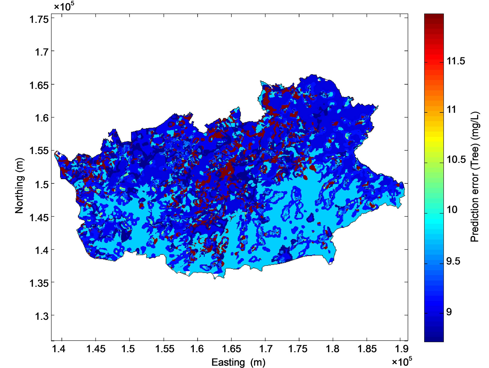 (b)
(b)
Figure 6. Map of groundwater nitrate concentration predicted by the regression tree model (a) and associated prediction error (b). The monitoring stations are symbolized by circles on (a).
 (a)
(a)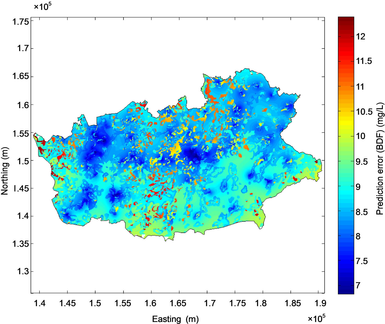 (b)
(b)
Figure 7. Map of groundwater nitrate concentration predicted by BDF (a) and associated prediction error (b). The monitoring stations are symbolized by circles on (a).
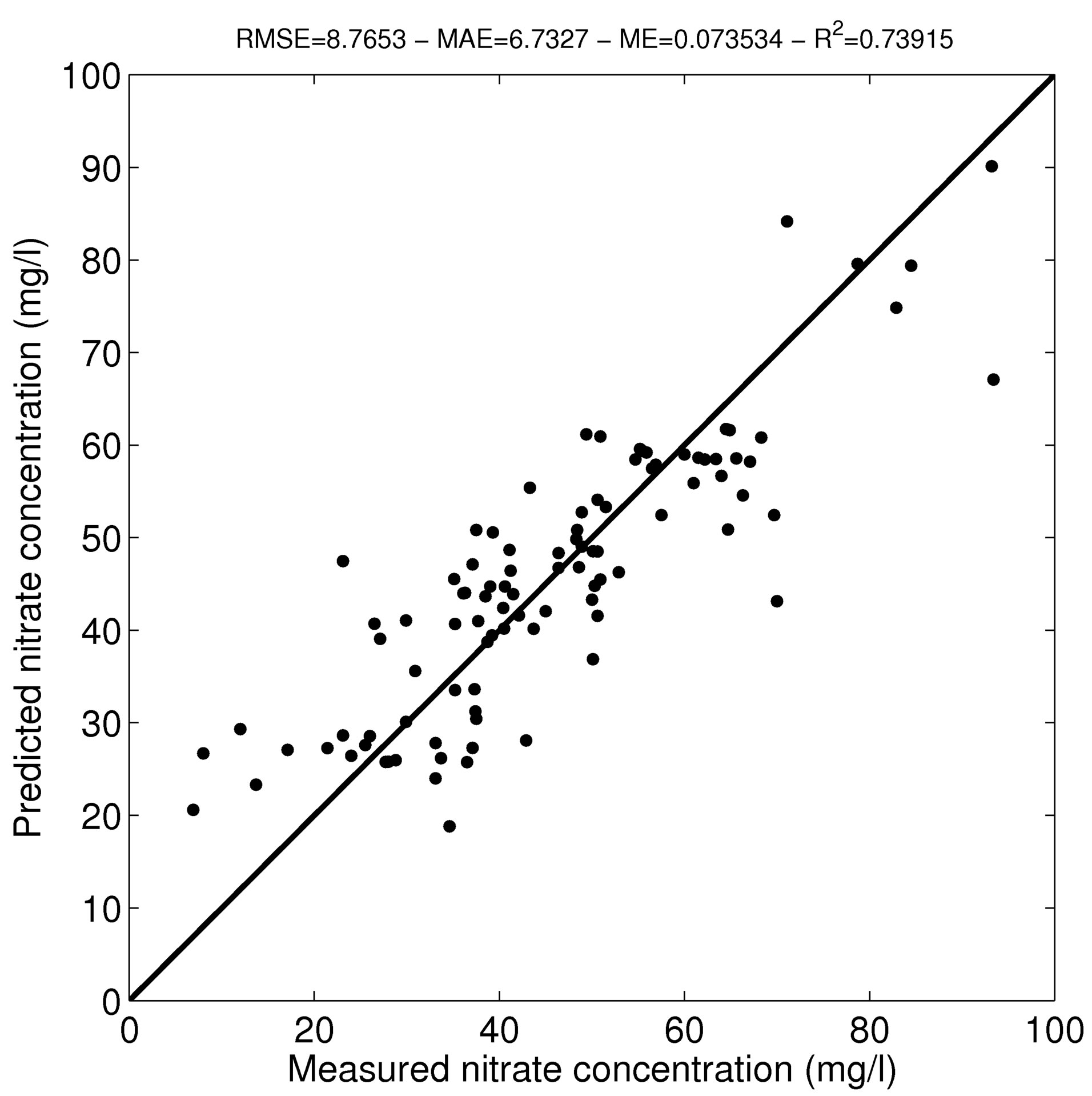
Figure 8. Comparison of the nitrate concentrations predicted by BDF to the measured nitrate concentrations. The plain line represents the 1:1 line.
gation in the aquifer makes the identification of a causal relationship not trivial.
Nitrate concentrations predicted with BDF have a mean regional value of 44.4 mg/L. The highest concentra-tions are observed in the agricultural regions of the center and east of the study area and in the north-west urban areas.
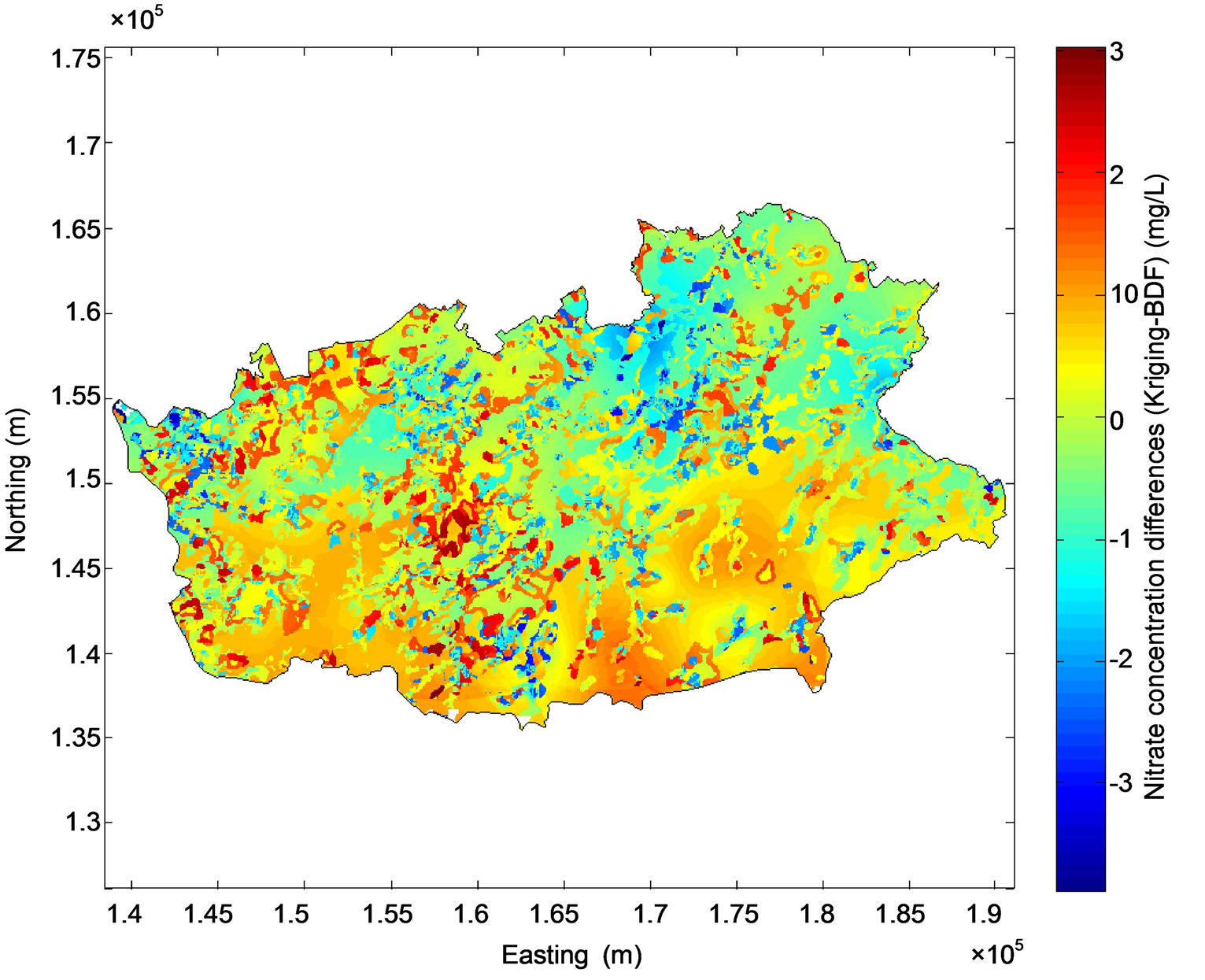
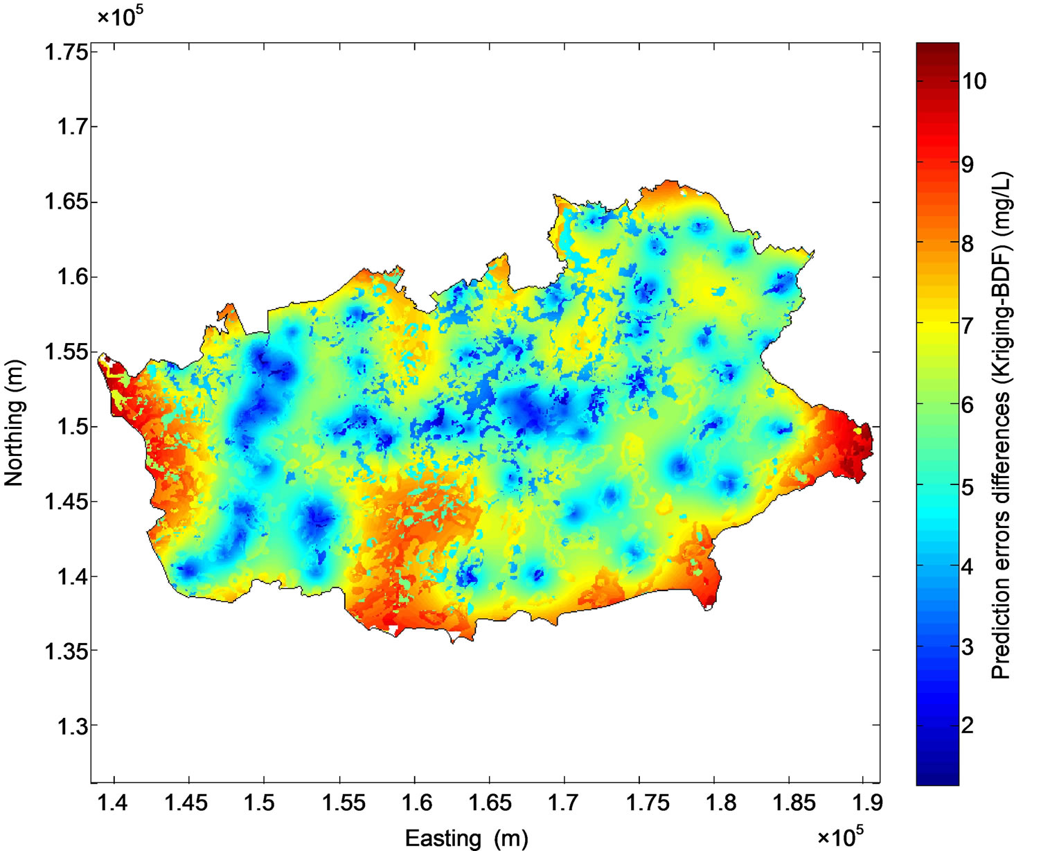
It is worth noting that the quality indicators used to compare the enhancement of the results of the three models are valid only at the regional scale and they do not permit to emphasize the detailed improvements of the mapping technique at the local scale. For this reason, the differences between the results of the various models were mapped. It can be observed from Figure 9(a) that large differences between kriged nitrate concentrations and concentrations predicted by BDF (from nearly −4 to 3 mg/L) appear between the two maps. Furthermore, Figure 10(a) shows that BDF reduces the uncertainty up to 10 mg/L in the regions where the monitoring network is scarce.
Also Figure 9(b) shows that the differences between nitrate concentrations predicted by the regression tree model and concentrations predicted by BDF vary between −2.5 and nearly 2 mg/L. These differences are located at proximity of the monitoring stations where the weight given to the kriged concentrations in the BDF process is higher than the weight of the concentration predicted by the regression tree model. Figure 10(b) shows that BDF reduces the uncertainty up to nearly 4 mg/L in the regions where the monitoring network is scarce, compared to the regression tree. As a conesquence, BDF has reduced prediction error compared both to kriging and the regression tree model and, in that sense, is an improvement for the mapping process.
It has been shown that the associated prediction uncertainty in the final map is smaller than those for the kriged map or the map predicted with the statistical model. This is a direct consequence that, under the assumption that all the distributions are Gaussian, the variance of the fused distribution is always smaller than each of the original distributions. This property has been shown in details in [15], Section 3.3.
The method is especially useful when information that has to be combined has prediction errors of the same order of magnitude. If not, the BDF map will be very similar to the map with the lowest uncertainty.
6. Conclusions
Groundwater contamination of the Brusselian sands (Belgium) by nitrate was mapped using a Bayesian Data Fusion framework, by combining groundwater monitoring data with a statistical groundwater contamination model. Nitrate concentrations measured in January and February 2009 were first spatialized over the whole study area using ordinary kriging. Since the monitoring stations are irregularly distributed in the study area, the kriging predictions have huge uncertainties where the density of monitoring stations is low. The monitoring stations network was not initially intended for environmental monitoring. Its low density in some places explains these large uncertainties.
In a second step, nitrate contamination was estimated using a statistical regression tree model. The predictions made by the regression tree have more homogeneous uncertainties throughout the study area. However, the nitrate concentrations measured at the monitoring stations do not appear on the map, since the regression tree is not an exact predictor.
In a third step, Bayesian Data Fusion allows combining the nitrate concentrations estimated by the interpolation method with those estimated by the statistical model into a single final map by weighting these estimates in terms of the associated uncertainty, thereby allocating a high weight to estimates which are very certain and a low weight to those that are very uncertain. It has been shown that the associated prediction uncertainty in the final map is smaller than those for both the kriged map and the map predicted with the statistical model.
In this case study, only two sources of information were combined to assess the nitrate pollution of the groundwater body at a given moment in time. Yet, the formal Bayesian Data Fusion framework allows integrating easily other data and could therefore be used to update the estimated map when new monitoring and modeling data about the status of the groundwater body
 (a)
(a)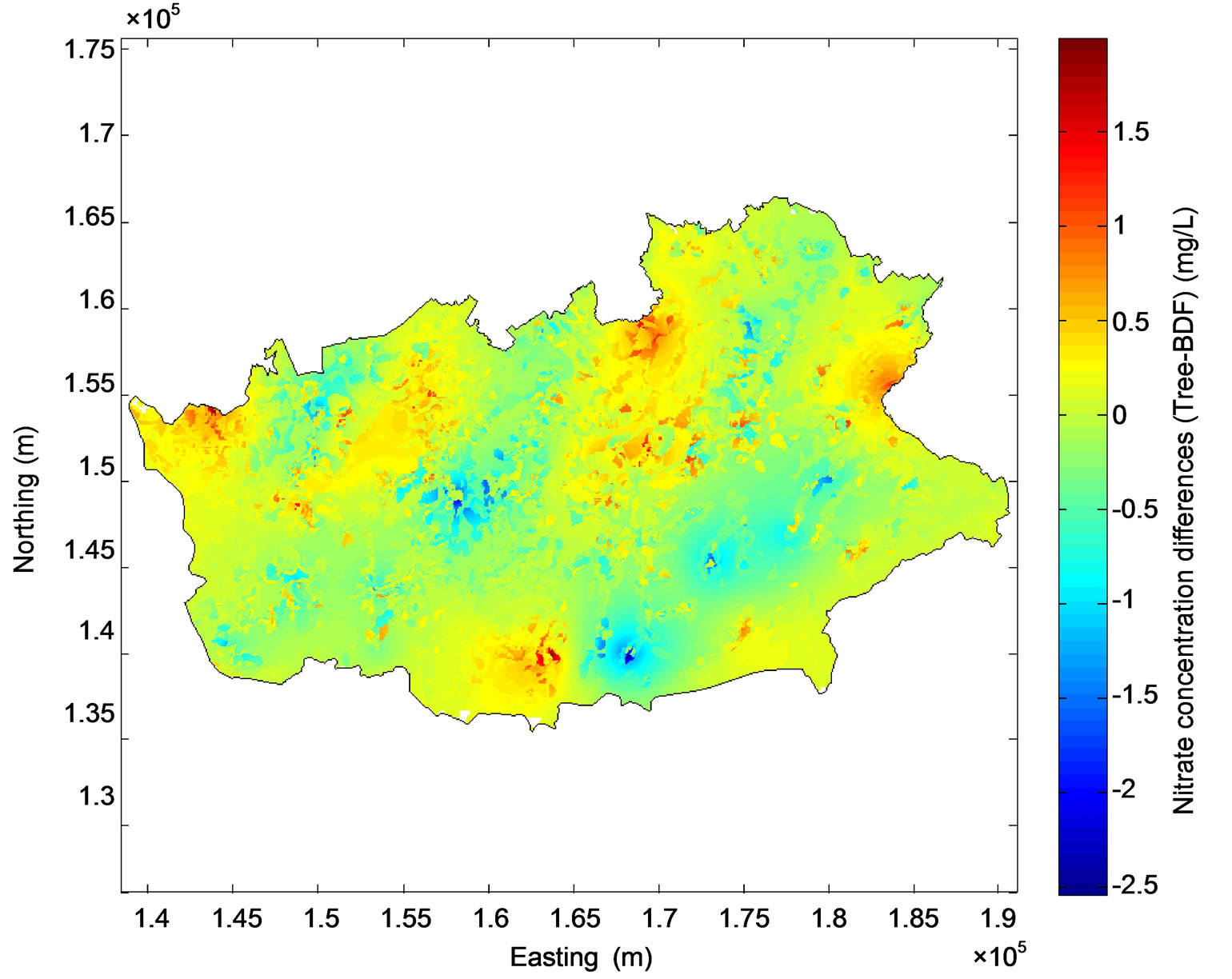 (b)
(b)
Figure 9. Differences between nitrate concentrations predicted by kriging and BDF (a) and between the regression tree model and BDF (b).
 (a)
(a)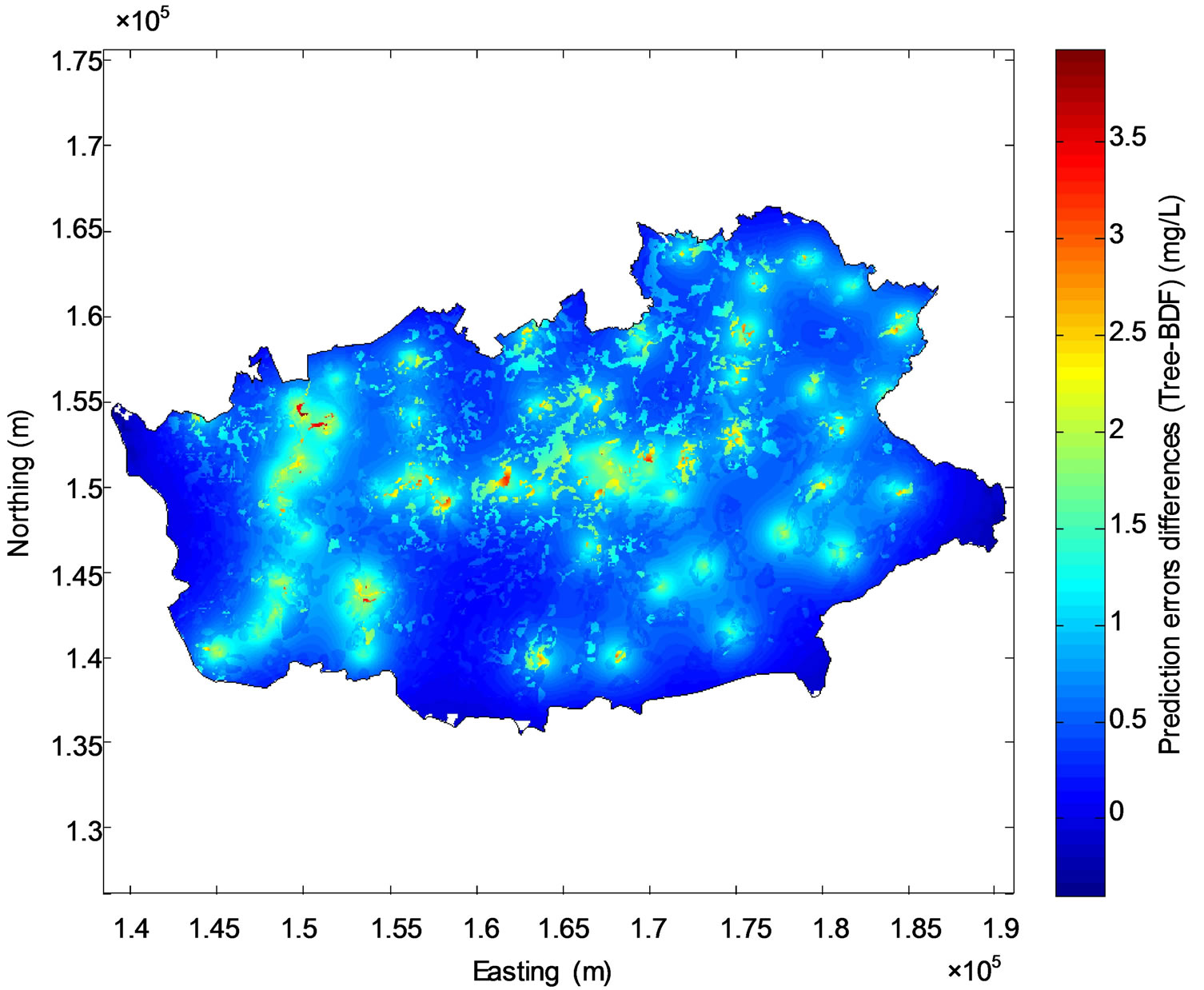 (b)
(b)
Figure 10. Differences between kriging prediction errors and BDF prediction errors (a) and between the regression tree prediction errors and BDF prediction errors (b).
becomes available. Hence, Bayesian Data Fusion is considered to be appropriate to generate updated high quality maps of the groundwater contamination at the regional scale.
Such updated high quality maps of groundwater contamination represent a powerful tool which could be used by the regional administration and the water production companies to implement specific and local water management and protection strategies. Increasing the density of the measurement network in the study area and using multilevel sampling tools would enhance the quality of the (geo)statistical analysis.
7. Acknowledgements
The reported work was funded by the “Fonds pour la formation à la Recherche dans l’Industrie et dans l’Agriculture” (FRIA, Belgium). The authors are grateful to the Service public de Wallonie (SPW) for providing them with land use and elevation maps.
REFERENCES
- “Directive 2000/60/EC Establishing a Framework for Community Action in the Field of Water Policy,” The European Parliament and Council Official Journal of the European Communities, L327/1, 2000.
- K. Hu, Y. Huang, H. Li, B. Li, D. Chen and R. E. White, “Spatial Variability of Shallow Groundwater Level, Electrical Conductivity and Nitrate Concentration, and Risk Assessment of Nitrate Contamination in North China Plain,” Environment International, Vol. 31, No. 6, 2005, pp. 896-903. doi:10.1016/j.envint.2005.05.028
- S. Fetouani, M. Sbaa, M. Vanclooster and B. Bendra, “Assessing Ground Water Quality in the Irrigated Plain of Triffa (North-East Morocco),” Agricultural Water Management, Vol. 95, No. 2, 2008, pp. 133-142. doi:10.1016/j.agwat.2007.09.009
- S. Cinnirella, G. Buttafuoco and N. Pirrone, “Stochastic Analysis to Assess the Spatial Distribution of Groundwater Nitrate Concentrations in the Po Catchment (Italy),” Environmental Pollution, Vol. 133, No. 3, 2005, pp. 569- 580. doi:10.1016/j.envpol.2004.06.020
- G. Christakos, P. Bogaert and M. Serre, “Temporal GIS. Advanced Functions for Field-Based Applications,” Springer, New York, 2002.
- S. Mattern, P. Bogaert and M. Vanclooster, “Introducing Time Variability and Sampling Rate in the Mapping of Groundwater Contamination by Means of the Bayesian Maximum Entropy (BME) Method,” In: L. Candela, I. Vadillo and F. J. Elor, Eds., Advances in Subsurface Pollution of Porous Media—Indicators, Processes and Modelling: IAH Selected Papers, Volume 14 (IAH—Selected Papers on Hydrogeology), Taylor and Francis, 2008, pp. 53-68.
- B. Duc, E. S. Bigün, J. Bigün, G. Maître and S. Fischer, “Fusion of Audio and Video Information for Multi Modal Person Authentication,” Pattern Recognition Letters, Vol. 18, No. 9, 1997, pp. 835-843. doi:10.1016/S0167-8655(97)00071-8
- A. Ross and A. Jain, “Information Fusion in Biometrics,” Pattern Recognition Letters, Vol. 24, No. 13, 2003, pp. 2115-2125. doi:10.1016/S0167-8655(03)00079-5
- G. D. Jones, R. E. Allsop and J. H. Gilby, “Bayesian Analysis for Fusion of Data from Disparate Imaging Systems for Surveillance,” Image and Vision Computing, Vol. 21, No. 10, 2003, pp. 843-849. doi:10.1016/S0262-8856(03)00071-4
- F. Cremer, K. Schutte, J. G. M. Schavemaker and E. den Breejen, “A Comparison of Decision-Level Sensor-Fusion Methods for Anti-Personnel Landmine Detection,” Information Fusion, Vol. 2, No. 3, 2001, pp. 187-208. doi:10.1016/S1566-2535(01)00034-3
- X. B. Song, Y. Abu-Mostafa, J. Sill, H. Kasdan and M. Pavel, “Robust Image Recognition by Fusion of Contextual Information,” Information Fusion, Vol. 3, No. 4, 2002, pp. 277-287. doi:10.1016/S1566-2535(02)00092-1
- X. E. Gros, J. Bousigue and K. Takahashi, “NDT Data Fusion at Pixel Level,” NDT & E International, Vol. 32, No. 5, 1999, pp. 283-292. doi:10.1016/S0963-8695(98)00056-5
- S. Y. Sohn and S. H. Lee, “Data Fusion, Ensemble and Clustering to Improve the Classification Accuracy for the Severity of Road Traffic Accidents in Korea,” Safety Science, Vol. 41, No. 1, 2003, pp. 1-14. doi:10.1016/S0925-7535(01)00032-7
- G. Simone, A. Farina, F. C. Morabito, S. B. Serpico and L. Bruzzone, “Image Fusion Techniques for Remote Sensing Applications,” Information Fusion, Vol. 3, No. 1, 2002, pp. 3-15. doi:10.1016/S1566-2535(01)00056-2
- P. Bogaert and D. Fasbender, “Bayesian Data Fusion in a Spatial Prediction Context: A General Formulation,” Stochastic Environmental Research and Risk Assessment, Vol. 21, No. 6, 2007, pp. 695-709. doi:10.1007/s00477-006-0080-3
- D. Fasbender, J. Radoux and P. Bogaert, “Bayesian Data Fusion for Adaptable Image Pansharpening,” IEEE Transactions on Geoscience and Remote Sensing, Vol. 46, No. 6, 2008, pp. 1847-1857. doi:10.1109/TGRS.2008.917131
- D. Fasbender, D. Tuia, P. Bogaert and M. Kanevski, “Support-Based Implementation of Bayesian Data Fusion for Spatial Enhancement: Applications to ASTER Thermal Images,” IEEE Geoscience and Remote Sensing Letters, Vol. 5, No. 4, 2008, pp. 598-602. doi:10.1109/LGRS.2008.2000739
- D. Fasbender, L. Peeters, P. Bogaert and A. Dassargues, “Bayesian Data Fusion Applied to Water Table Spatial Mapping,” Water Resources Research, Vol. 44, No. 12, 2008, Article ID: W12422. doi:10.1029/2008WR006921
- L. Peeters, D. Fasbender, O. Batelaan and A. Dassargues, “Bayesian Data Fusion for Water Table Interpolation: Incorporating a Hydrogeological Conceptual Model in Kriging,” Water Resources Research, Vol. 46, 2010, pp. 8532-8532. doi:10.1029/2009WR008353
- D. Fasbender, O. Brasseur and P. Bogaert, “Bayesian Data Fusion for Space-Time Prediction of Air Pollutants: The Case of NO2 in Belgium,” Atmospheric Environment, Vol. 43, No. 30, 2009, pp. 4632-4645. doi:10.1016/j.atmosenv.2009.05.036
- IBW—Intercommunale du Brabant Wallon, “Étude des Ressources en Eau du Brabant Wallon,” Contrat Région Wallonne, 1987.
- PCNOSW, Projet de Cartographie Numérique de L’occupation du Sol de Wallonie, “Projet Notifié par le Gouvernement Wallon,” Faculté Universitaire des Sciences Agronomiques de Gembloux, 2005.
- F. A. Baker, D. L. Verbyla, C. S. Hodges and E. W. Ross, “Classification and Regression Tree Analysis for Assessing Hazard of Pine Mortality Caused by Heterobasidion Annosum,” Plant Disease, Vol. 77, No. 2, 1993, pp. 136- 139. doi:10.1094/PD-77-0136
- B. G. Lees and K. Ritman, “Decision-Tree and RuleInduction Approach to Integration of Remotely Sensed and GIS Data in Mapping Vegetation in Disturbed or Hilly Environments,” Environmental Management, Vol. 15, No. 6, 1991, pp. 823-831. doi:10.1007/BF02394820
- H. A. J. Vanlanen, C. A. Vandiepen, G. J. Reinds and G. H. J. Dekoning, “A Comparison of Qualitative and Quantitative Physical Land Evaluations, Using an Assessment of the Potential for Sugar-Beet Growth in the European Community,” Soil Use and Management, Vol. 8, No. 2, 1992, pp. 80-89. doi:10.1111/j.1475-2743.1992.tb00899.x
- M. J. Crawley, “Statistics, an Introduction Using R,” Wiley, New York, 2005.
- J. J. Rothwell, M. N. Futter and N. B. Dise, “A Classification and Regression Tree Model of Controls on Dissolved Inorganic Nitrogen Leaching from European Forests,” Environmental Pollution, Vol. 156, No. 2, 2008, pp. 544-552. doi:10.1016/j.envpol.2008.01.007
- S. Mattern, D. Fasbender and M. Vanclooster, “Discriminating Sources of Nitrate Pollution in an Unconfined Sandy Aquifer,” Journal of Hydrology, Vol. 376, No. 1-2, 2009, pp. 275-284. doi:10.1016/j.jhydrol.2009.07.039