Journal of Software Engineering and Applications
Vol.6 No.7(2013), Article ID:33795,5 pages DOI:10.4236/jsea.2013.67044
Using Genetic Algorithms for Solving the Comparison-Based Identification Problem of Multifactor Estimation Model
![]()
1Computer Engineering Department, University of Jordan, Amman, Jordan; 2Computer Science Department, Kharkov National University, Kharkov, Ukraine.
Email: sweidan@ju.edu.jo, tps_kharkov@mail.ru, dimetroid@yandex.ru
Copyright © 2013 Andraws Swidan et al. This is an open access article distributed under the Creative Commons Attribution License, which permits unrestricted use, distribution, and reproduction in any medium, provided the original work is properly cited.
Received April 23rd, 2013; revised May 25th, 2013; accepted June 2nd, 2013
Keywords: genetic algorithm; comparatory identification; fitness-function; chromosome; crossover; mutation
ABSTRACT
In this paper, the statement and the methods for solving the comparison-based structure-parametric identification problem of multifactor estimation model are addressed. A new method that combines heuristics methods with genetic algorithms is proposed to solve the problem. In order to overcome some disadvantages of using the classical utility functions, the use of nonlinear Kolmogorov-Gabor polynomial, which contains in its composition the first as well as higher characteristics degrees and all their possible combinations is proposed in this paper. The use of nonlinear methods for identification of the multifactor estimation model showed that the use of this new technique, using as a utility function the nonlinear Kolmogorov-Gabor polynomial and the use of genetic algorithms to calculate the weights, gives a considerable saving in time and accuracy performance. This method is also simpler and more evident for the decision maker (DM) than other methods.
1. Introduction
Identification of the object mathematical model is to determine its parameters based on experimental investigation of the object. Identification is the most time-consuming and very important operation in the synthesis model.
The classical problem of identification is to determine the mathematical model y = F(x) of the object which consists of determining the transformation rules of the input x into output y or more precisely the form and parameters of operator F. Such identification is called direct because it is based on direct quantitative measurement of input and output signals of the object. However, in some cases, there is a need to identify an object, when the researcher has no direct access to information about the output signal. The objects considered in this paper, are assumed to be of this type.
In different situations, estimates given by the person to one or other properties of an object are subjective and cannot be directly measured by any physical devices. In such cases, the classical methods of the direct identification are not applicable. Alternative methods are indirect identification. The most convenient and widely used among these methods is the comparison-based identification [1].
2. Statement of the Problem
Suppose we have a set of alternatives (solutions) X = {xj},  , each of which is characterized by a set of individual criteria (characteristics) ki,
 . The values of individual criteria
  are clearly defined. Based on the analysis of this information a person shall select the most preferred solution from the set of solutions X, for example
 , i.e. he sets strict order relation on the set of alternatives X:
 .
.
It means that, according to the utility theory [2], which postulates the existence of scalar quantify the preference of any alternative  we can write:
 , (1)
, (1)
where —individual scalar evaluation of the usefulness of the alternatives.
On the basis of this information it is necessary to synthesize the mathematical model of individual choice of the decision maker, i.e, a model of generalized utility formation .
.
Currently, the most widely used two forms of utility functions are: the additive:
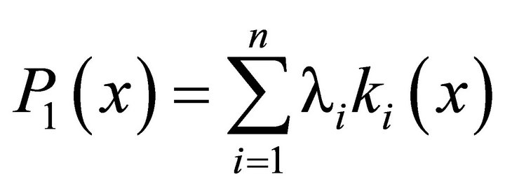 (2)
(2)
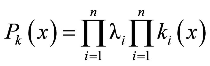
and multiplicative:
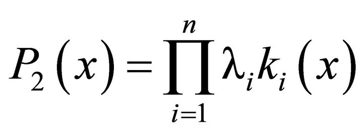 (3)
(3)
where λi isomorphism coefficients indicating dimension, significance, possible values range, partial criteria ![]() that lead to the isomorphism type.
that lead to the isomorphism type.
The most informative situation is one in which the coefficients of isomorphism are given numerically. Since λi is a constant, then (3) can be rewritten as follows:
 (4)
(4)
Analysis of (4) shows that the multiplicative estimation does not take into account the “weights” of partial criteria, since the product  is a constant scaling multiplication factor and does not affect the relationship of different solutions
 . Therefore, additive utility function is more universal and widely used.
Equation (2) makes sense only if  takes into account the importance of individual criteria and are at the same time isomorphism coefficients. Most often, defining such coefficients is a big problem, so it was decided to represent the additive utility function in the form:
 (5)
(5)
where —dimensionless relative weight coefficients that satisfy the following restrictions:
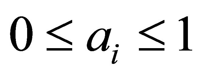 ,
, 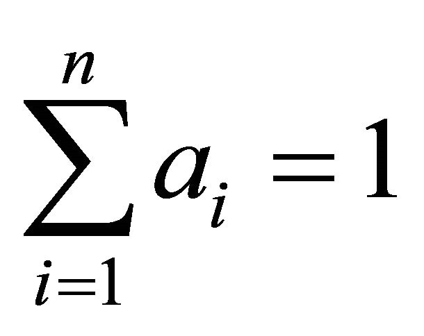 , (6)
, (6)
and  is normalized, i.e. transformed to the isomorphic type partial criteria.
The normalization is performed by the following formula:
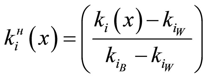 (7)
(7)
where —value of the private criteria;
 ,
, — the best and worst value (accordingly) of the private criteria that is among the domain of admissible values.
In such a way the problem of utility function synthesis reduces to the parametric identification of the relative importance coefficients. Expert evaluation methods or comparison-based identification methods are used for this purpose [3].
An additive utility function disadvantage is that it does not consider the possible nonlinear dependence of the utility function on the individual criteria absolute values ![]() and their mutual influence.
and their mutual influence.
Great theoretical and practical interest is the solution of the general structure-parametric identification problem of the individual evaluation model under less restrictive assumptions about the structure of the model.
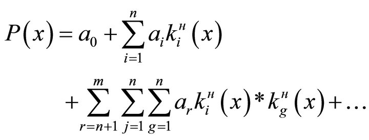
For this purpose the Kolmogorov-Gabor polynomial is suggested as a possible structure class.
 , (8)
, (8)
and genetic algorithms as a method for solving the general structure-parametric identification problem.
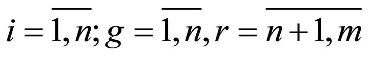
This approach allows us to describe any nonlinear dependence and does not impose any apriority restrictions on the additive or multiplicative utility functions, since polynomial (8) contains in its composition the first as well as higher degrees of characteristics  and all their possible combinations.
3. Optimal Complexity Model Definition
The aim of the solution the comparatory structure-parametric identification problem is to synthesize an optimal complexity model, which provides the minimum error of approximation criteria of experimental data output model.
Any sequence of N experimental data can be accurately approximated by an N − 1 degree polynomial by solving a system of normal algebraic equations. However, this approximation does not mean that an adequate, high accuracy model with good prognostic features is synthesized. This is due to the fact that experimental data contain measurement and other uncontrolled random errors. Therefore, the polynomial of high complexity, not only approximates the desired signal, but random errors of experimental data as well. To overcome this drawback in [3,4] splitting the sample of experimental data into two sets of data: training and testing is proposed. The first subset is used for the synthesis of the model and determine its characteristics, for example the method of least squares, and the second—to check the accuracy of the model. It was found that increasing the complexity of the model improves the accuracy of approximation of the test sequence of the experimental data until it reaches a minimum, and then begins to decline due to the inclusion of “harmful” random components. Model, which gives a minimum test sequence approximation error, was named as the optimal complexity model [3].
This raises the problem of choosing criteria of accuracy evaluation of the mathematical model. In the case of the classical identification the most commonly used criteria is the least squares, for the implementation of which numerical input and output experimental data is necessary. In the case of identification of multifactor estimation model, as noted above, quantitative information about the output effects is not available. In this regard, a number of specific problems, considered below, came to the surface.
4. Solving the Comparatory Identification Problem by the Genetic Algorithms Method
In the above formulation, the comparatory structure-parametric identification problem can be solved by different methods and algorithms. But common to all of them is the need to implement a sequence of procedures:
• generation of the model structure;
• defining the quantitative values of its parameters;
• assessing the quality of the model.
Various combinations of algorithms, of different precision, complexity, versatility, for the first and second stages are possible. To obtain perfectness and versatility evaluation criteria in the field of the methods application there is a need for their investigation. With the help of computer experiments genetic programming algorithms were synthesized and investigated.
Genetic Algorithms (GAs) are based on the mechanisms of natural selection and implement a scheme of “survival of the fittest” among the considered structures, shaping and changing the search algorithm based on modeling the evolution of search. In each generation a new set of artificial sequences is created using part of the old set and the addition of new parts with “good properties” [5-9].
GA starts with a random set of solutions called population. Each element of the population is called a chromosome and represents a solution to the problem. The chromosomes evolve over multiple iterations, bearing the name of generations. In the process of iteration chromosome is estimated using the fitness-function [6,7,10].
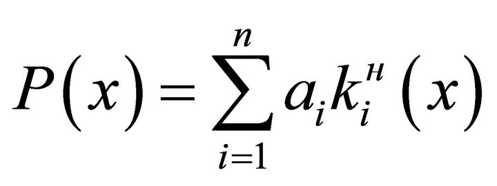
In solving the problem of structure-parametric identification on the first step a population of chromosomes, describing the structure of the model is created. This is done by selecting a class of admissible structures. Kolmogorov-Gabor polynomial, taking out the free term and limiting it to only linear and quadratic terms (squares and pair wise combinations of variables), was chosen as this class. Then the polynomial will be written as follows:
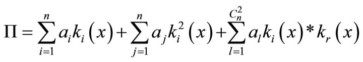
 (9)
(9)
It means that for n partial criteria the complete polynomial will have
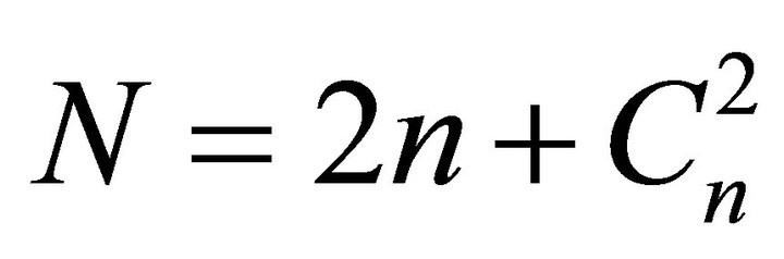 (10)
(10)
terms, where  is the number of combinations and is equal to:
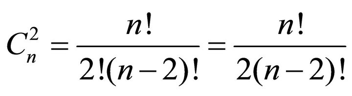 (11)
(11)
Consequently, each chromosome of the population must contain N bits.
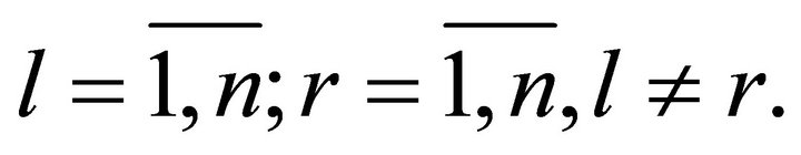
The validity of imposing such limitations on the complexity of the polynomial is based on the fact that after the normalization by formula (7) all partial characteristics have values . Squaring these numbers or the multiplication of any two of them lead to a rapid decrease in the values. In addition, each term of the polynomial is multiplied by a coefficient
(because ).
).
Based on the fact that the calculation of utility function  and weights
  with accuracy higher than two decimals is impractical, it can be concluded that it is impractical as well to include terms higher than the second order.
After the generation of the chromosomes population, which describes the model structure, in the second stage, for each of them, a parametric identification is provided by one of the following possible methods:
• Method of determining the Chebyshev point on the polyhedron described by the system of inequalities  ,
,  [5];
[5];
• The genetic algorithms method.
The first of these methods is described in [2,5] and will not be considered. The implementation of the genetic algorithm is as follows. For each chromosome of the population, which characterizes a model structure, we determine the number  of coefficients
  equal to the number of units in the chromosome. By definition, the coefficients must satisfy the following conditions:
 ,
, (12)
(12)
and is expressed to two decimal places. Hence the number of bits that must contain the chromosome of each coefficient is equal to [8,10]:
![]() , (13)
, (13)
where [ai, bi]—interval range of , pointed in (12), and resultant chromosome of all the coefficients ai,
  is
is
 (14).
(14).
For each chromosome of the structure population we form population of chromosomes coefficients ai and solve the problem of the genetic selection of these coefficients values that maximize the match function. As a match function the number of satisfied inequalities of (9) can be taken. If necessary it can be divided into training and testing sets.
On the established populations an iterative procedure of genetic selection on the first and second populations to achieve the best value of the match function is implemented.
Example: Let us assume a situation where a decision maker has to choose the best option among five alternatives of computer systems with four partial criteria: processor frequency, memory size, hard disk capacity and price.
The decision maker represents the situation by constructing Table 1.
After that the maximum and minimum values of each criterion are defined and the quantitative normalized partial criteria are calculated by formula 7.
As a result of the above mentioned operations we get table 2 which represents the set of the alternatives with their normalized partial criteria.
Next, the DM selects the best, in his opinion, alternative. Let us assume that the DM chooses the fourth alternative. Next step is to calculate the additive utility function. First the weight coefficients are calculated and then inserted in the linear Kolmogorov-Gabor polynomial. Thus the additive utility function is expressed as:
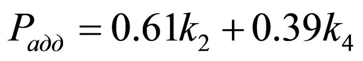 (15)
(15)
We start the procedure of genetic algorithms.
Let there be two chromosomes: a parent that contains the complete Kolmogorov-Gabor polynomial (Figure 1), and a child that contains only the components of the first term (Figure 2).
Child chromosome will be for us the resultant, which is the shortest polynomial satisfying the condition
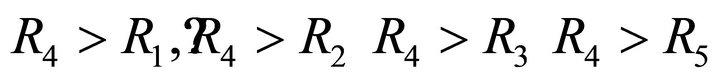 (16)
(16)
This condition (16) will be the criterion on which we will carry out the selection.
Next, using the above mentioned method of genetic algorithms to solve the comparison-based structural-parametric identification we get variant of a child chromosome that meets criterion (16).
The next step is to choose an optimal length utility function represented as the Kolmogorov-Gabor polynomial. That is, the shortest polynomial that satisfies (16)
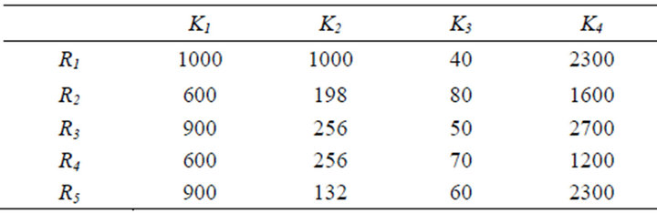
Table 1. The set of alternatives with their partial criteria.
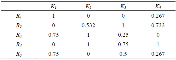
Table 2. Alternatives with normalized criteria.

Figure 1. parent chromosome.

Figure 2. child chromosome.
and at the same time has the maximum utility function. To do this, we introduce one more condition:
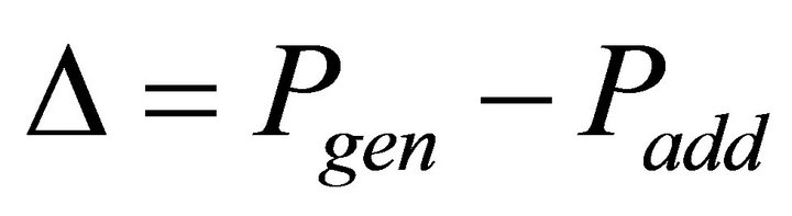 ,
, (17).
(17).
Thus, after finding the optimal length KolmogorovGabor polynomial satisfying (16), we check that polynomial. For the chosen alternative substituting partial criteria we obtain the following lengths:
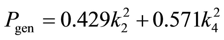 (18).
(18).
Hence the utility functions of the different alternatives are: R4 = 1; R3 = 0.429; R2 = 0.4277; R5 = 0.04; R1 = 0.04.
The utility function of alternative R4 is maximum, and other alternatives are worse and thus the problem is correctly solved.
5. Conclusion
The use of nonlinear methods for the identification of the multifactor estimation model showed that the use of a new technique, using as a utility function the nonlinear Kolmogorov-Gabor polynomial and the use of the genetic algorithms to calculate the weights gives a considerable saving in time and accuracy performance. It is as well simpler and more evident for the decision maker than other methods.
REFERENCES
- A. O. Ovezgeldyev and K. E. Petrov, “Comparatory Identification of Linear Multifactor Estimation Models Parameters,” Radioelektronika i Informatika, Vol. 2, No. 3, 1998, pp. 41-43.
- A. O. Ovezgeldyev, E. G. Petrov and K. E. Petrov, “Synthesis and Identification of Multifactor Estimation and Optimization Models,” Naukova Dumka, Kiev, 2002, 161 p.
- G. K. Voronovsky, К. V. Machotilo, S. N. Petroshev and S. А. Sergeev, “Genetic Algorithms, Artificial Neural Networks and Virtual Reality Problems,” Osnova, Kharkov, 1997, 112 p.
- V. М. Kureychik, “Genetic Algorithms. State. Problems,” Teoriya i Systemy Upravleniya, No. 1, 1999, pp. 144-160.
- E. G. Petrov and Д. А. Булавин, “Application of Chebyshev’s Dot and Genetic Algoritms’ Methods for Determination the Structure of Multifactor Estimation Model,” Problemy Bioniki, No. 58, 2003, pp. 36-44.
- E. G. Petrov and Д. А. Булавин, “Application of Genetic Algoritms’ Method for Solving the Multifactor Estimation Model Comparatory Identification Problem,” Radioelektronika i Informatika, No. 1, 2003, pp. 89-93.
- J. Zhang, H. Chung and W. L. Lo, “Clustering-Based Adaptive Crossover and Mutation Probabilities for Genetic Algorithms,” IEEE Transactions on Evolutionary Computation, Vol. 11, No. 3, 2007, pp. 326-335. doi10.1109/TEVC.2006.880727
- L. M. Schmitt, “Theory of Genetic Algorithms II: Models for Genetic Operators over the String-Tensor Representation of Populations and Convergence to Global Optima for Arbitrary Fitness Function under Scaling,” Theoretical Computer Science, Vol. 310, No. 1, 2004, pp. 181- 231. doi10.1016/S0304-3975(03)00393-1
- D. Goldberg, “Genetic Algorithms in Search, Optimization and Machine Learning,” Addison-Wesley Professional, Reading, 1989.
- А. P. Rotshteyn, “Intelligent Identification Technologies,” Universum-Vinnica, Vinnica, 1999, 320 p.