Journal of Biomedical Science and Engineering
Vol.6 No.4(2013), Article ID:30500,13 pages DOI:10.4236/jbise.2013.64057
Comparing biomarkers and proteomic fingerprints for classification studies
![]()
1Advanced Biomedical Computing Center, Information Systems Program, SAIC-Frederick, Inc., Frederick National Laboratory for Cancer Research, Frederick, USA
2Laboratory for Surgical Research, Department of Surgery, University Hospital Schleswig-Holstein, Campus Luebeck, Luebeck, Germany
3Laboratory of Proteomics and Analytical Technologies, Advanced Technology Program, SAIC-Frederick, Inc., Frederick National Laboratory for Cancer Research, Frederick, USA
4Genetics Branch, National Cancer Institute, NIH, Bethesda, USA
Email: lukebria@mail.nih.gov
Copyright © 2013 Brian T. Luke et al. This is an open access article distributed under the Creative Commons Attribution License, which permits unrestricted use, distribution, and reproduction in any medium, provided the original work is properly cited.
Received 4 January 2013; revised 5 February 2013; accepted 21 February 2013
Keywords: Biomarker; Classifier; Proteomic Fingerprint
ABSTRACT
Early disease detection is extremely important in the treatment and prognosis of many diseases, especially cancer. Often, proteomic fingerprints and a pattern recognition algorithm are used to classify the pathological condition of a given individual. It has been argued that accurate classification of the existing data implies an underlying biological significance. Two fingerprint-based classifiers, decision tree and medoid classification algorithm, and a biomarker-based classifier were examined using a published dataset of mass spectral peaks from 81 healthy individuals and 78 individuals with benign prostate hyperplasia (BPH). For all three methods, classifiers were constructed using the original data and the data after permuting the labels of the samples (BPH and healthy). The fingerprint-based classifiers produced accurate results for the original data, though the peaks used in a given classifier depended upon which samples were placed in the training set. Accurate results were also obtained for the dataset with permuted labels. In contrast, only three unique peaks were identified as putative biomarkers, producing a small number of reasonably accurate biomarker-based classifiers. The dataset with permuted labels was poorly classified. Since fingerprint-based classifiers accurately classified the dataset with permuted labels, the argument for biological significance from a fingerprint-based classifier must be questioned.
1. INTRODUCTION
It is well established that early detection of cancer has a positive effect on treatment and longevity. Historically, the prediction of the presence of a disease has relied on measuring the concentration of a particular protein or biomarkers, such as prostate specific antigen (PSA) for prostate cancer and cancer antigen (CA)-125 for ovarian cancer. The low sensitivity and/or specificity of these biomarkers necessitate the search for new biomarkers, but the discovery of new biomarkers has been exceedingly slow. Bioinformatic analysis of data obtained from biofluids, such as the undirected search of spectral peaks from samples of blood, urine, tears, mucous, and spinal fluid may be extremely useful in identifying new biomarkers. Unfortunately over 4000 publications have “identified biomarkers” in the last 7 - 10 years, but none have been FDA approved. This suggests that it is possible to correctly classify the available samples without reflecting the underlying biology of the disease.
Informatic analysis has led to a new paradigm for classification known as fingerprinting or pattern matching. In this paradigm, individuals are classified based upon a particular pattern of intensities. If an untested individual has the same pattern as an individual with a known condition, then these two are given the same disease classification. Commonly used fingerprint-based classifiers include decision trees [1-4] and the medoid classification algorithm [5-10] used by the laboratories of Petricoin and Liotta.
Sufficient classification of a training dataset and a “blinded” validation set by a fingerprinting classifier is commonly used as the basic justification that this particular classifier must be based on some underlying biological principal [11]. If a three-node decision tree (Figure 1) was selected as the classifier, and was deemed biologically relevant because it sufficiently classified a training set and a validation set of individuals, then one would have to perform an exhaustive search of all possible three-node decision trees with all possible cut points to determine if any other classifiers performed with sufficient accuracy (sensitivity = specificity = 90% in this hypothetical example). If no others were found, then the argument about biological relevance may have merit. If more than one were found, then the question of why all are biologically relevant remains.
If a fingerprinting classifier is found that performs extremely well on classifying the training data, but classifies the validation data poorly, one can either state that the classifier is insufficient and therefore not biologically relevant, or that there was an incorrect separation of training and validation data so that all important fingerprints were not present in the training data. Since the discriminating fingerprints are not known, proper coverage cannot be known, and therefore proper selection of the training data cannot be known. In addition, since the quality of classifying the validation set is the metric used to determine biological relevance, the validation set is used in the process of constructing the classifier and is therefore part of the training process.
With these points in mind, an effective way to construct classifiers based on fingerprints is to include all data in the search for fingerprinting classifiers and then to selectively remove samples for the testing set in a way that preserves the coverage of the fingerprint in the training data. This statement does not suggest, in any way, that this procedure has been used by other research groups who present fingerprinting classifiers; it simply states that this method is an effective way to ensure that all required fingerprints are present in the training data.
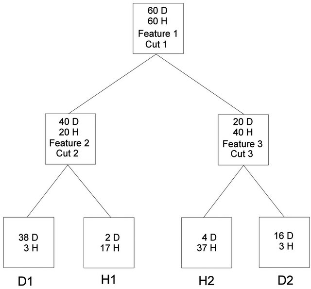
Figure 1. Hypothetical decision tree.
In addition, the significance of a fingerprinting classifier needs to be established. Permutation testing is often used to test significance. In this investigation, the phenotypes were scrambled amongst all data to determine if a new classifier of the same form (e.g. a three-node decision tree) could be constructed with comparable accuracy. The probability that random phenotypes could be classified to a given accuracy determines the significance of a given model.
In this study, the publicly available data set used by Adam et al. [12] to identify proteomic fingerprints that are diagnostic for prostate cancer was examined. In particular, spectra from individuals with benign prostate hyperplasia (BPH) were compared to spectra from “healthy” individuals without BPH or prostate cancer. Instead of using specific or binned mass-to-charge (m/z) intensities, a peak-picking algorithm was used to select 158 intensity maxima in non-overlapping regions of the spectra, and these intensity maxima were used in attempts to classify the BPH and healthy individuals using both the true phenotypes and datasets where the phenotypes have been randomly scrambled.
These datasets were examined using two fingerprinting algorithms, a decision tree (DT) and a medoid classification algorithm (MCA). In all known applications of a decision tree to produce a classifier using spectral data [1-4], a single scoring metric (e.g. Gini Index, entropy gain, etc.) was used to determine the cut point at a given node so that the two daughter nodes were as homogeneous as possible (e.g. diseased versus healthy). The procedure used here was to construct unconstrained decision trees that best classify the training and testing individuals. A wrapper algorithm was used to determine which features and cut points are to be used in a putative DT classifier and the goal was to optimize the overall sensitivity and specificity.
The medoid classification algorithm was a best attempt at reproducing the algorithm used in many of the studies conducted in the laboratories of Emmanuel Petricoin and Lance Liotta [5-10]. As opposed to the method used in the references cited above, this investigation will fix the number of features that are present in the classifier. Again, a wrapper algorithm is used to determine which features will be used in a putative classifier.
The original and permuted datasets were also examined using a biomarker-based classifier embodied in the Biomarker Discovery Kit (BMDK) [13]. A suite of filtering algorithms were used to search for putative biomarkers, and then only these peak intensities were used in a final classifier based on a distance-dependent K-nearest neighbor (DD-KNN) algorithm. This was different from the program that previously identified a form of C3a found in the blood as a marker for individuals with colorectal cancer and benign polyps [14]. In this earlier investigation, both filter and wrapper algorithms were used to identify putative biomarkers, while this investigation only used an expanded set of filtering algorithms.
The next section outlines the procedures used to prepare the datasets and construct classifiers for each of the three methods. This explanation is followed by a section that describes the classification of both the true and scrambled phenotypes using each method and the fourth section contains a discussion of these results and is followed by the overall conclusions of this analysis.
2. METHODS
2.1. Dataset Preparation
The spectra produced by Adam et al. [12] were from 78 individuals with BPH and 81 healthy individuals. The raw data contained intensities (ion counts) at 48,538 m/z values from −0.0991 to 198,660. The dataset contained two spectra that were acquired from each individual. As outlined in the colorectal study [14], the peak-picking process initially truncated each spectrum to 17,686 m/z values from 1500 to 40,500 and then scaled these intensities such that their sum (total ion current) is 50,000. The BPH and healthy spectra were randomly divided into two groups; a training set that contained 104 BPH spectra (duplicate spectra from 52 individuals) and 108 healthy spectra (duplicates from 54 individuals), and a testing set that contained the remaining 52 BPH (26 duplicates) and 54 healthy (27 duplicates) spectra.
The 212 training spectra were averaged together such that the intensity at each m/z value was the average of the intensities across the 212 spectra. This average training spectrum was examined to find the m/z value with the highest intensity, which was placed in a peak list. All intensities at m/z values within 0.3% of the selected value were set to zero and the process was repeated until the selected intensity was less than 25% of the average intensity (below 0.707); at which point the process stopped. This processing produced 424 m/z values where the average training spectrum contained sufficient intensity for further examination. Each of these was taken as the center of a spectral region with a half-width of 0.15% of the m/z where the individual spectra may have contained a peak, a shoulder region, or a nondescript flat region of sufficient intensity. To reduce this list further, each of these regions in the 212 training spectra were examined and a region was kept if the maximum intensity was not in the first two or last two m/z values in at least 60% of either the BPH or healthy spectra. This process reduced the number of spectral regions to 158. These 158 regions were examined in each of the training and testing spectra, and the maximum intensity within that region was recorded.
The final step was to average the intensities between the two spectra from each individual for each of the 158 regions. Therefore, the final datasets contained the averaged maximum intensities in 158 regions. The training set contained the averaged intensities for 52 BPH and 54 healthy individuals while the testing set contained averaged intensities for 26 BPH and 27 healthy individuals.
2.2. Classifier Construction
Two different procedures can be used to determine which peak intensities, or features, are used in the classifier; one uses a wrapper algorithm and the other uses one or more filtering algorithms. A wrapper algorithm uses an external stochastic or deterministic algorithm to select putative features that are used in the final classifier. Once the search for putative feature sets is complete, one or more final classifiers are produced. In contrast, a filtering method uses one or more independent procedures to search for discriminating features, and only these features are used in the final classifier. It is important to note that the filtering algorithms should not use the same procedure used in the final classifier. Both DT and MCA fingerprint-based classifiers used a wrapper algorithm to search for the best set of features (and cut points for the DT method), while BMDK used a filter method to first search for putative biomarkers.
2.3. Decision Tree Classifier
Two different procedures were used to construct unrestricted decision trees. For the symmetric, 3-node decision tree in Figure 1, all possible feature triplets were used in all six combinations and all possible cut points were examined. The possible cut points were determined by ranking the intensity of a given feature from lowest to highest and then selecting the average of consecutive intensities. The score for a given decision tree was the sum of the sensitivity and specificity for the training data in the four terminal nodes.
For the symmetric, 7-node decision tree shown in Supplemental Figure 1, a modified Evolutionary Programming (mEP) procedure [15] was used. Each putative decision tree classifier was represented by two 7-element arrays; the first contained the feature used at each node and the second contained the cut values. Both arrays assumed the node ordering listed in Supplemental Figure 1. The only caveats were that all seven features must be different and that this ordered septet of features was not the same as any other putative solution in either the parent or offspring populations. When a new putative decision tree was formed, a local search was used to find optimum cut points for this septet of features.
The mEP procedure started by randomly generating 2000 unique decision trees. Each decision tree had one or two of the features removed and unique features were selected, again requiring that the final septet was unique. The local search first tried to find optimum cut points for the new features that were added and then the search was performed over all seven cut points. The best set of cut points was combined with the septet of features to represent an offspring classifier. The score was again the sum of the sensitivity and specificity for the training individuals over the eight terminal nodes. When the entire set of initial, or parent, decision trees generated unique offspring, all 4000 scores were compared and the 2000 decision trees with the best score became parents for the next generation. This process was repeated for a total of 4000 generations and the best classifiers in the final population are examined. Each time a decision tree was constructed during the mEP search, each decision node was examined. If the number of either BPH or healthy samples was a given number (denoted NSTOP) or less, it became a terminal node and the feature for this node and any subsequent nodes (for nodes 2 and 3) were removed. Each time a tree was truncated, all offspring generated from this solution also had this truncation.
2.4. Medoid Classification Algorithm
While the algorithm described by Petricoin and Liotta [5-10] used a genetic algorithm driver to search for an optimum set of features, allowing for different putative solutions to use different numbers of features (5 - 20 features), our algorithm used a mEP feature selection algorithm and all putative solutions had the same number of features n. For a given value of n, n features were selected and the intensities of these features were rescaled for each individual using the following formula [5-10]:
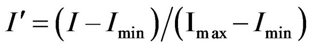
In this equation, I is a feature’s original intensity, I' is it’s scaled intensity, and Imin and Imax are the minimum and maximum intensities found for the individual among the n selected features, respectively. If Imin and Imax were from the same features in all samples, a baseline intensity would be subtracted and the remaining values scaled so that the largest intensity was 1.0. Each individual would then be represented as a point in an (n − 2)-dimensional unit cube. As designed, and as found in practice, Imin and Imax do not represent the same features from one individual to the next, so this interpretation does not hold. Therefore, each individual represents a point in an n-dimensional unit cube.
The first training sample became the medoid of the first cell, with this cell being classified as the category of this sample. Each cell had a constant trust radius r, which was set to 0.1 (n)1/2, or ten percent of the maximum theoretical separation in this unit hypercube. If the second sample was within r of the first, it was placed in the first cell; otherwise it became the medoid of the second cell and that cell was characterized by the second sample’s category. This iteration continued until all training samples were processed. Each cell was then examined and the categories of all samples in the cell were compared to the cell’s classification. This calculation allowed a sensitivity and specificity to be determined for the training data, and their sum represented the score for this set of n features.
The mEP algorithm initially selected 2000 sets of n randomly selected features. The only caveat was that each set of n features must be different from all previously selected sets. The medoid classification algorithm then determined the score for each set of features. Again, each parent set of features generated an offspring set of features by randomly removing one or two of the features and replacing them with randomly selected features, requiring that this set be different from all feature sets in the parent population and in all offspring generated so far. The score of this feature set was determined and the score and feature set was stored in the offspring population. After all 2000 offspring had been generated the parent and offspring populations were combined. The 2000 feature sets with the best score were retained and became the parents for the next generation.
It should be noted that for a set of n features, the number of unique cells that can be generated is on the order of 10n. Since no training set is ever this large (n is 5 or more), only a small fraction of the possible cells will be populated and classified. As will be shown in the next section, this limitation caused a significant number of the testing samples to be placed in an unclassified cell, though none of the publications that used this method [5-10] reported an undetermined classification for any of the testing samples. Instead of searching through a large number of solutions that classified the training samples to a significant extent and find those that minimized the number of unclassified testing samples, we decided to use all samples and limit the number of cells. All samples were placed in the training set and the algorithm was run with the added requirement that any set of n features that produced more than 52 BPH cells or 54 healthy cells was given a score of zero. As long as the number of cells that used a BPH sample as the medoid was 52 or less, and the number of cells with a healthy medoid was 54 or less, it was possible to select the medoid samples as the training set. All other samples could then be divided to place the required number in the testing set and the remainder would be part of the training set.
This restriction also allowed for a test of the dependence of the result on the order of the samples. In one run the order of the samples was the 52 BPH training samples, the 54 healthy training samples, the 26 BPH testing samples and then the 27 healthy training samples. In the second case, the order of these four sets was reversed.
2.5. Biomarker Discovery Kit
In contrast to an earlier version of BMDK [14], 10 different filtering methods are employed to identify any putative biomarkers [13]. Each of the methods (described in detail in Supplemental Methods) examined each of the 158 features and selected those features that produce the best scores. In general, five features were selected by each method, but this was increased if multiple features produced the same good score. Once all features were selected, the Pearson correlation coefficient was determined between all feature pairs and features were placed in the same group if r > 0.70. This was done so that at most one putative biomarker can be selected from each group. The raw spectrum around the selected features in each group, and any other feature with r > 0.70 to a selected feature, was visually examined to ensure that it was a well-defined peak (obtained from a single protein, protein complex, or fragment). If more than one welldefined peak existed within a single group, the peak with the highest maximum intensity became the putative biomarker.
The putative biomarkers were then used in a distancedependent 6-nearest neighbor classification algorithm (DD-6NN). This algorithm, also described in detail in Supplemental Methods, weighed the probability that a test sample had the same classification as one of its neighbors by the inverse of the distance to this neighbor. This procedure also included the ability to classify a sample as “undetermined” if it was sufficiently far from all of its neighbors.
A Euclidean distance was used to determine the separation between a selected sample and a neighbor sample. If more than one peak was used in the classifier, a peak with a high maximum intensity had a larger effect on the distance than one with a small maximum intensity. Therefore, the final classifier was constructed using the unscaled peak intensities and the peak intensities after they had been scaled by dividing by the standard deviation across all samples used in constructing the classifier.
3. RESULTS
3.1. Original Data
The 10 methods within BMDK identified a total of nine features in the training set that may represent putative biomarkers (Table 1). The intensities of the feature at m/z 4072.8 correlated with those at m/z 8137.9 across all training samples (r > 0.70). In addition, the intensities at m/z 7198.5, 8294.5, and 8359.9 also sufficiently correlated with at least one of these features, and this fivefeature set was denoted Group 1. The four selected features at m/z 4475.2, 4579.1, 8942.8, and 9149.0 correlated strongly with each other and none of the other features, so they are combined into Group 2. The selected feature at m/z 4876.0 correlated with the feature at m/z 4860.6 to form Group 3, the selected feature at m/z 5740.3 correlated with features at m/z 5978.0 and 6122.4 to form Group 4, and the selected feature at m/z 9662.3 correlated with features at m/z 9430.7 and 9729.3 to form Group 5. The original spectra was examined around each of these 17 m/z values to determine if it represented an isolated peak that is produced by a single protein, protein complex, or fragment. Five of the 17 features represented well-defined peaks; one from Group 1, two from Group 2, and two from Group 4 (Supplemental Table 1). For the two groups containing a pair of well-defined peaks, the intensities of these peaks were examined and the peak with the highest maximum intensity was selected for use in the DD-6NN classifier. The intensities of the three selected peaks (m/z 4072.8, 6122.4 and 8942.8) are shown in Figure 2. This figure shows that the peaks at m/z 4072.8 and 8942.8 have significantly higher intensity in many of the BPH samples (left column) than for the healthy samples (right column). In addition, the peak at m/z 8942.8 corresponds to the blood form of complement C3a anaphylatoxin (C3a-desArg) that represented the observed biomarker for individuals with colorectal cancer and polyps [14].
A separate analysis of all samples (combining the training and testing sets) selected seven features (Supplemental Table 2) which correlated into three groups. A visual examination of these seven features and all correlated features identified the same three peaks as putative biomarkers shown in Figure 2 (Supplemental Table 3); reinforcing the robustness of these markers.
All combinations of one, two, and three peak intensities were used in the DD-6NN classifier, revealing the classification accuracies shown in Tables 2(a) and (b).
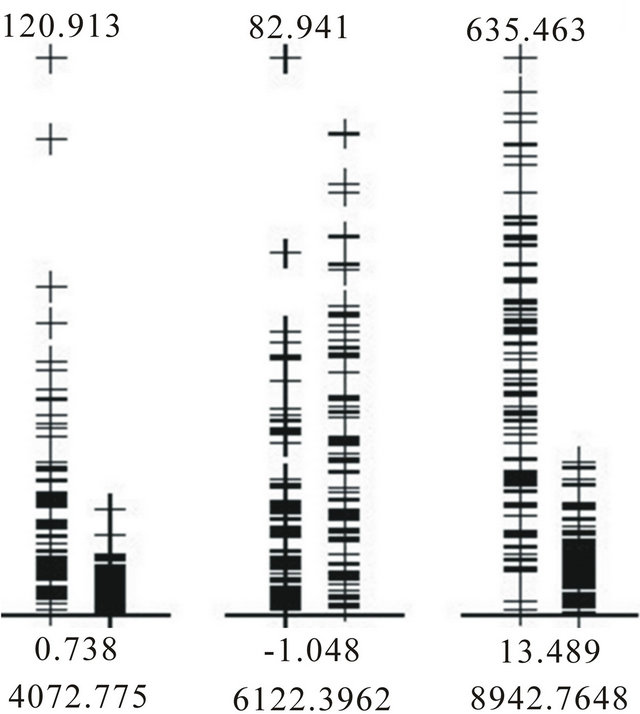
Figure 2. Intensities of the BPH (left column) and healthy (right column) samples in the training dataset for each of the three putative biomarkers.
Table 1. Nine features selected by the 10 different filtering methods in BMDK for the training set using unpermuted phenotypes. The numbers in each column are the ranks of the features for each method.
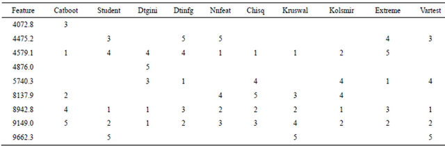
Table 2. Results of the classification of BPH versus healthy samples using the true phenotypes: (a) Best DD-6NN classification results using only the three putative biomarkers shown in Figure 2 and an unscaled Euclidean distance; (b) Best DD-6NN classification results using only the three putative biomarkers shown in Figure 2 and a scaled Euclidean distance; (c) Quality of the final 2000 classifiers using all samples in a symmetric 7-node decision tree; (d) Number of perfect MCA classifiers (sensitivity = specificity = 100%) and times particular peaks were used in them.
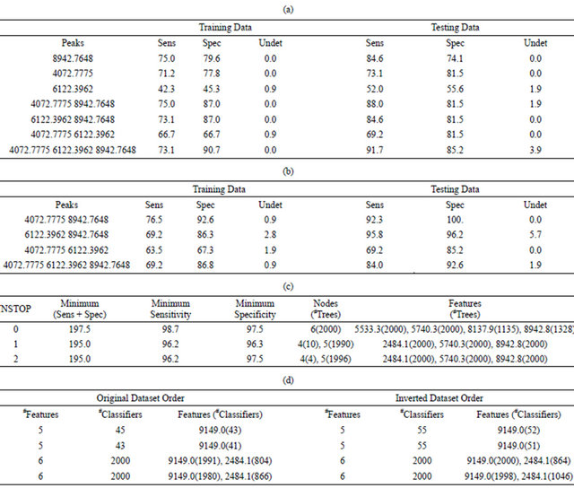
Table 3. Results of the classification of BPH versus healthy samples using the true phenotypes: (a) Sensitivity and specificity of the best DD-6NN classifiers using between one and three putative biomarkers for the training dataset using an unscaled Euclidean distance; (b) Sensitivity and specificity of the best DD-6NN classifiers using between one and three putative biomarkers for the training dataset using a scaled Euclidean distance; (c) Average quality (%) of the classification using a symmetric 7-node decision tree for the best and 200th best solution for eight different runs when either all samples are used in the training (All) or when the score is the average of the sensitivity and specificity for both the training and testing sets (Avg); (d) Specific DT results for the best results from the fourth and seventh All runs; (e) Sensitivity and specificity of the best and 100th best medoid classifier for each of two runs where the number of features (#F) was varied from five to eight and the classifier was required to have at most 52 BPH cells and 54 healthy cells and regularly used features.
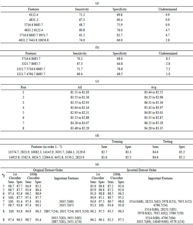
The results in Table 2(a) are obtained if the Euclidean distance between a pair of samples uses the unscaled intensities. The best two-feature classifier used the peaks at m/z 4072.8 and 8942.8. There was an imbalance in the contribution of these peaks to the distance since the C3a peak at m/z 8942.8 had a maximum intensity of 635.5 while the peak at m/z 4072.8 had a maximum intensity of only 120.9 (Figure 2). In order to equalize their contribution to the classifier the intensities of each peak were first scaled by the inverse of the standard deviation as determined by the training samples. This produced the results in Table 2(b) and showed an increase in the accuracy of this classifier for both the training and testing data.
An exhaustive search for symmetric 3-node decision trees was conducted with the requirement that the training set had a sensitivity and specificity of 94% or more. This search identified a total of 12,344 unique decision trees, meaning that they all had different features and/or cut points. It should be noted that the discriminating peaks at m/z 4072.8 and 8942.8 represent a total of nine features since they are members of groups that contain five and four features, respectively (Supplemental Table 1). Of the 12,344 unique 3-node decision trees producing a sensitivity and specificity of 94% or more for the training set, 1653 trees did not use any of the nine features from these two groups. Therefore, it is possible to obtain good results for the training set without using the putative biomarkers.
The 3-node decision tree with the best results for the training set (sensitivity = 98.1%, specificity = 98.1%) only produced a sensitivity of 81.5% for the testing set. This suggests that a necessary piece of the underlying fingerprint was missing from this decision tree. Therefore, all samples were used to construct decision trees that contained up to seven decision nodes (Supplemental Figure 1).
Running the mEP search for 4000 generations with a population size of 2000 produced the results listed in Table 2(c) for the final population of 2000 unique decision trees. Here the uniqueness was over features, meaning that no two trees could have the same features at the same nodes, independent of the cut points used.
When NSTOP = 0, the minimum value of (sensitivity + specificity) was 197.5% across all 2000 decision trees, while the minimum values for the sensitivity and specificity were 98.7% and 97.5%, respectively, in any given tree. All 2000 final trees contained six decision nodes, and the intensities at m/z of 5533.3 and 5740.3 were used in all 2000 trees. The peak intensity for m/z of 8942.8 was used in 1328 trees while m/z of 8137.9 was used in 1135 trees. When NSTOP was increased to one, the minimum (sensitivity + specificity) was 195.0% for all 2000 decision trees, while no tree had a sensitivity or specificity below 96.2% or 96.3%, respectively. Note that 10 of these decision trees used only four decision nodes while the remaining 1990 trees used five decision nodes. This means that 4000 unique decision trees were constructed in these two runs.
The medoid classifier algorithm started with searches that used four features, which is smaller than the number considered by the groups of Petricoin and Liotta [5-10]. Forty-four different combinations were found to produce 100% sensitivity and specificity for the training data. The best result for the testing data (sensitivity = 100%, specificity = 95.0%) used features at m/z of 2484.1, 2589.7, 4876.0, and 9149.0, but caused 18.9% of the testing individuals to receive a classification of “unknown”. The classifier that minimized the number of “unknowns” used a completely different set of features at m/z of 4072.8, 7480.3, 7935.3, and 9300.8. It yielded an “unknown” classification for only two testing samples (1.8%), but caused the sensitivity for the testing set to drop to only 40%. In addition, two of the 44 sets of four features did not include any of the nine features from the groups that contained the putative biomarkers at m/z 4072.8 and 8942.8.
When five features were used in this classifier, the mEP algorithm produced a final population where all 2000 of the unique feature sets produced a 100% sensitivity and specificity for the training data. This result means that there were at least 2000 5-feature MCA classifiers that yielded perfect training results. One could search through all possible results to find the ones that performed sufficiently well on the testing data; or one could use the method described above to ensure coverage of any identified fingerprint in the training set.
When all data were placed in the training set, two mEP run found 43 and 45 different sets of five features, respectively, that produced perfect results without forming more than 52 BPH cells and 54 healthy cells (Table 2(d)). Both mEP runs using six features produced final populations of 2000 unique feature sets that produced overall sensitivities and specificities of 100%. When the order of the datasets was reversed, both 5-feature mEP runs produced 55 models that perfectly classified all of the data. If six features were used in the classifier, all 2000 members of the final population produced 100% sensitivities and specificities in both mEP runs.
3.2. Permuted Phenotypes
The BPH/healthy classifications were randomly scrambled between the 106 training individuals and independently scrambled between the 53 testing samples. This process ensured that the same peak intensities were present in the training and testing sets.
When the 10 filtering methods in BMDK examined this dataset with no biological information, 25 features were selected (Supplemental Table 4). A correlation analysis caused these 25 peaks to form 19 groups. Instead of visually inspecting the original spectra about each of these 25 features, and all features that correlated with them, the feature from each group with the highest maximum intensity was selected for use in a DD-6NN classifier. The 19 selected features are shown with an asterisk in Supplemental Table 4 and their intensities are displayed in Supplemental Figure 2. As expected, none of the features shown in the figure represented a strong putative biomarker.
A search over all possible combinations of one, two and three features produced the classification results for the training data shown in Tables 3(a) and (b). The classification accuracies for the training data using either unscaled intensities (Table 3(a)) or intensities scaled by the standard deviation (Table 3(b)) were definitely worse than the results shown in Tables 2(a) and (b) for the unpermuted phenotypes.
A symmetric 7-node decision tree (Supplemental Figure 1) was again used to classify the data. If the tree was constructed just using the testing data, a large number of unique trees produced good sensitivity and specificity. In one run, all 200 of the top trees had an average quality that was above 88%. Unfortunately, the quality on the training set was generally not any better than a random guess (as expected). To see if decision trees could be built that effectively classified both the training and testing data, two different methods were employed to promote fingerprint coverage in the training set. The first (denoted All) simply combined all data into the decision tree, allowing one to manually extract the training set after the tree was built. This had the advantage that it had the best possible coverage of a given fingerprint. The second method (denoted Avg) was to augment the score of a given decision tree so that it was the average of the sensitivity and specificity for both the training and testing sets. This method had the advantage that the division between training and testing was fixed, but effectively weighed the testing results twice as much as in the All runs.
The mEP feature selection algorithm was run eight times with different seeds to the random number generator to produce the average sensitivity and specificity for the best and 200th best solution, as shown in Table 3(c). For the All runs, these numbers are the average sensitivity and specificity for the decision trees that processed all of the data, but it is easy to extract a testing set from all individuals such that the training and testing qualities are approximately equal. For example, Table 3(d) lists the features in order for the best decision trees from the fourth and seventh All runs, along with sensitivities and specificities after 26 BHP and 27 healthy individuals were extracted to form a testing set. Though the qualities of these decision trees were very similar, and very good considering the fit was to random phenotypes, the features used in each tree were quite different. The feature at m/z 2 823.9 was the only one appearing in both trees, but in the first decision tree it separated those samples who have a low intensity at m/z 13 574.7 while in the second it treated individuals with high intensities in m/z 14 925.8 and 3 824.5.
The Avg results in Table 3(c) were the average sensitivities for both the training and testing sets. The higher quality results were due to a larger weight of the testing data relative to the training data. For example, the best result from the third Avg run had a sensitivity and specificity of 78.8 and 85.2% for the training data, respectively, but 92.3 and 88.9%, respectively, for the testing data. The reported Avg value was simply (78.8 + 85.2 + 92.3 + 88.9)/4.0 = 86.3, the average of these percentages. If the same model was used to produce an All result, the sensitivity and specificity of the training data would have twice the weight and the score would be determined from the equation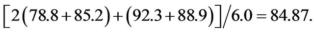 Note that this All score was worse than the corresponding Avg score, but better than any of the All results listed in Table 3(c). This was likely due to a better search over features, and particularly the cut points, when a smaller training set was used in the Avg runs. Therefore, while the results in Table 3(c) are good, better results should be possible if a more extensive search was performed, especially for the All runs.
When the medoid classification algorithm was used to construct a classifier using all available data, the results in Table 3(e) are obtained. Again, the mEP search was run for 4000 generations and the population size was 2000 putative models, requiring that the final classifier does not contain more than 52 BPH cells and more than 54 healthy cells. Table 3(e) lists the sensitivity and specificity of the best classifier and the 100th best classifier in the final population, as well as any features used in 50 or more of the top 100 classifiers. The number of features was varied from five to eight and each mEP search was run twice, with different seeds to the random number generator, using both the original order of the datasets, and these datasets in an inverted order.
Table 3(e) shows that a sensitivity and specificity of approximately 95% was obtained for the datasets with randomized phenotypes using only six features, and that many good results were obtained when more than six features were used.
4. DISCUSSION
This investigation used a dataset that contained only 158 features (peak intensities) and 159 samples from 78 individuals with BPH and 81 individuals with healthy prostates. The 10 filtering methods in BMDK identified three uncorrelated features (Figure 2) from a training set of 52 BPH and 54 healthy individuals. These three features were also identified from an examination of all 159 samples. After scaling the peak intensities by their standard deviation, the 2-feature DD-6NN classifier using the peaks at m/z of 4072.8 and 8942.8 performed better on both the training and testing sets than the classifier using all three putative markers (Table 2(b)). The DD-6NN classifier therefore has the property that using more features does not necessarily make the classifier better.
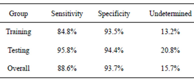
It should be stressed that other final classifiers could be used with the filtered putative biomarkers. For example, in the earlier study of colorectal cancer [14], the blood-based form of C3a (m/z 8942.8 in this study) was used in a simple decision rule using peak intensities and ELISA blood concentrations, like that shown in Figure 4. When this was done for BPH using all samples, an individual was predicted to have BPH if the intensity of this peak was above 138.0, with a sensitivity of 88.6% (Table 4). If this intensity was below 89.0, they were predicted to not have BPH with a specificity of 93.7%. An individual obtained an “unknown” classification about 16% of the time, and other procedures would have to be used to test for BPH.
After permuting the phenotypes, the filtering methods in BMDK identified 19 features (Supplemental Table 4), but none appeared to be a strong candidate as a biomarker (Supplemental Figure 2). Tables 3(a) and (b) show that no combination of one, two or three features was able to construct a DD-6NN classifier with an average sensitivity and specificity above 75%.
The DT and MCA fingerprint methods showed similar behavior for both the original dataset and the dataset after label permutations. For the dataset with correct phenotypes, an exhaustive search of symmetric 3-node decision trees identified 12,344 trees which fit the training data with a sensitivity and sensitivity of 94% or more. At least 2000 5-feature MCA classifiers fit the training data with a sensitivity and specificity of 100%. The purpose of the testing data would then be to determine which of these many classifiers contained the proper fingerprint; making the testing data part of the training proTable 4. Predicted results using the decision rules BPH if I(8942.8) > 138.0, healthy if I(8942.8) < 89.0, otherwise undetermined.
cess. In addition, many decision trees and MCA classifiers did not use any of the nine peaks associated with m/z 4072.8 or 8942.8, so good results were obtained for the training data without using one of the putative biomarkers identified by BMDK.
Since these results were for just a single division of the samples into a training set and a testing set, all such divisions would have to be examined. Instead, a short-cut method was used to identify classifiers that would fit both the “training” and “testing” sets. Over 4000 decision trees were produced that, using between 4 and 6 nodes, yielded a sensitivity and specificity of 96.2% or higher (Table 2(c)). In addition, 55 5-feature and at least 2000 6-feature MCA classifiers correctly classified all individuals (Table 2(d)).
It should be stressed that the “testing” set was strictly used to determine which of the thousands of classifiers that properly classified the “training” data also had high classification accuracies for the samples not used in the classifier construction. These thousands of qualifying classifiers have therefore never been validated. Any new sample would have to be independently analyzed and used to determine which of these classifiers still possessed the proper fingerprints and/or used in the training of new classifiers to incorporate any missing fingerprint. Therefore, this new sample would have to become part of the training process. Since this is a cyclic argument, no new sample could simply be tested and neither of these types of classifier could ever be generalizable [16, 17] to the entire population.
The results in Tables 3(c) and (e) show that very good results could be obtained for all of the available data when the phenotypes were scrambled. This is related to Ransohoff’s concept of chance [16,17], though differences do exist. Several symmetric 3-node decision trees and 4- feature MCA classifiers were able to accurately classify the training data without using any of the nine peaks that correspond to the putative biomarkers at m/z of 4072.8 and 8942.8. Therefore, a chance fitting to the data is the construction of a classifier that accurately fits the data without using a putative biomarker. If thousands of fingerprints can be generated for a given classification model, it is also highly unlikely that all of them have a biological basis. The present study shows that there was a problem with the flexibility of the classifier and its ability to fit random data. If the data is known to be random and the accuracy of the classifier is comparable to the accuracy using the initial data, then the classifier based on the initial data is not significant. This does not mean that the original data is necessarily random and does not contain putative biomarkers; it means that the proposed classifier is overly flexible and can produce good results using any dataset. It should also be emphasized that both the DT and MCA classifiers have the property that the classification accuracy cannot get worse across the population of putative classifiers if the number of features present in the classifier increases. Therefore, if the quality is insufficient, the investigator simply has to use more features in the classifier.
Since we have shown that it is impossible to produce a generalizable classifier using a fingerprint-based method, the “personalized medicine” approach [18-22] needs to be clarified. Stating that fingerprint-based classifiers should not be used does not imply that all BPH patients are necessarily the same. For example, a scatter plot of the best overall 2-feature DD-6NN classifier is shown in Figure 3. The feature at m/z 2633.8 was found to be a well-defined peak in those spectra with significant intensity, and those individuals with significant intensity all had low intensity in the m/z 8942.8 peak and predominantly had BPH. This classifier had a sensitivity and specificity of 84.6 and 94.4% for the training data and 88.5 and 88.9% for the testing data, respectively, with no undetermined individuals. This was better than the DD- 6NN results using m/z 8942.8 alone (Table 2(a)) and gives a specificity that was significantly better than the best result using two putative biomarkers. Since the peak around m/z 2633.8 had significant intensity for so few samples, it did not appear in enough models to be selected by BMDK.
The results in Figure 3 suggest two possibilities; either the improvement caused by including m/z 2633.8 in the classifier is due to chance [16,17] (i.e. a full analysis of a much larger population would show that m/z 2633.8 also has significant intensity in healthy individuals and/ or individuals with a high intensity in m/z 8942.8), or the BPH category is actually composed of two states (one
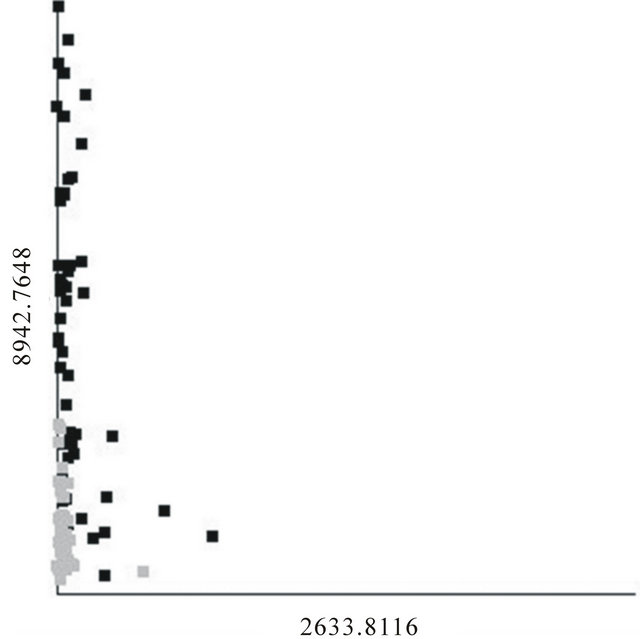
Figure 3. Scatter plot of the best 2-feature, 6-neighbor DD-KNN result for the BPH (black) and healthy (gray) individuals.
with a sufficient intensity in m/z 8942.8 and a second, smaller group with a sufficient intensity in m/z 2633.8). If the latter possibility turns out to be true, then one may well expect that any treatment for individuals in one BPH state would be different than that for those in the other BPH state.
Though it has been stated [23] that multiple biomarkers should be able to classify a set of samples better than a single biomarker, multiple markers should not be used in a concerted fashion, as in a fingerprint. Since a single disease may be composed of multiple states, genetic or proteomic markers would be needed to properly stratify the population and then use the biomarker appropriate for that state. If two or more biomarkers were used to distinguish samples in a single state, it would be difficult to determine if the markers were all dependent upon the state of the samples as opposed to correcting specific samples. For example, if a single state was represented by the samples shown in Figure 4, and one of the markers used in the classifier was the one shown in this figure, any other features could be used to distinguish those that are “undetermined” by this marker. Therefore these other features could be used to classify those specific samples with an intermediate intensity for the marker, and represents a fingerprint, or proteomic pattern, for these samples. Since fingerprint-based classifiers should be avoided, this is equivalent to stating that a classifier should not use features which predominantly act on a subset of samples within a single state. A later publication will describe a method for testing a classifier to determine the extent to which sample specific features are used.
5. CONCLUSIONS
These results showed that putative biomarkers obtained strictly from the training data using the filtering methods in BMDK were able to produce classifiers without the
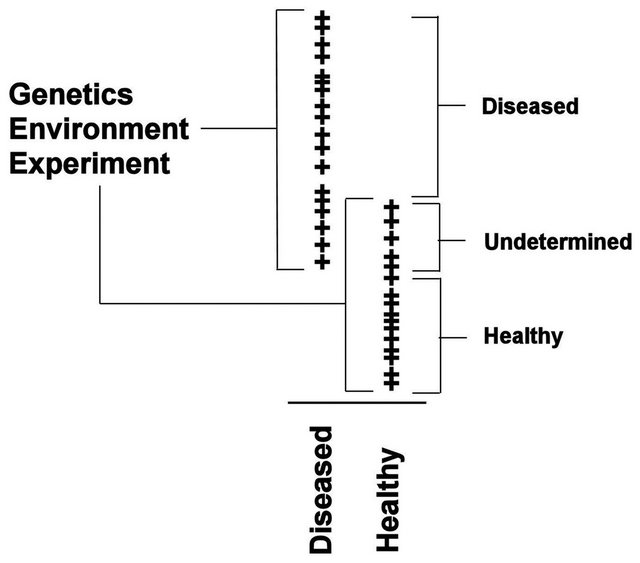
Figure 4. Peak intensity plots for a putative biomarker.
use of the testing data. Poor results for the training set were obtained when the phenotypes were scrambled; therefore significance is not a problem. As long as the experimental design does not introduce bias into the spectra, a biomarker-based classifier may be generalizable to the full population to the extent to which the known samples effectively cover the intensity range for the biomarkers.
A fingerprint-based classifier algorithm has particular problems with ensuring that there is sufficient coverage of viable fingerprints in the training data. An a priori division of the available data into a training set and testing set can hide a potentially viable fingerprint due to incomplete coverage. Fingerprint-based classifiers also have a problem with uniqueness since it is shown that a large number of classifiers are able to distinguish between individuals with BPH and those that are healthy. In addition, fingerprint-based classifiers of even a modest complexity were shown to classify a random dataset to a relatively high quality, causing significance to be a problem.
Coverage and uniqueness require that any new data must effectively be used as part of the training process; either to reduce the number of classifiers that produce sufficiently good results or to modify the existing classifiers because of insufficient coverage. Therefore, DT and MCA fingerprint-based classifier cannot be apriori generalizable to the full population.
Though the concept of “personalized medicine”, as is pertains to the use of protein fingerprints, is found to be invalid, the results presented here do suggest that a phenotypic category may be composed of more than one state. As shown in Figure 3, it may be possible that the BPH category represents two states and each state is identified by its own biomarker. Therefore, any classification algorithm should try to classify on a specific state, not on overall categories or personal fingerprints.
6. ACKNOWLEDGEMENTS
This project has been funded in whole or in part with federal funds from the National Cancer Institute, National Institutes of Health, under Contract NO1-CO-12400. The content of this publication does not necessarily reflect the views or policies of the Department of Health and Human Services, nor does mention of trade names, commercial products, or organizations imply endorsement by the United States Government.
REFERENCES
- Ho, D.W., Yang, Z.F., Wong, B.Y., Kwong, D.L., Sham, J.S., Wei, W.I., et al. (2006) Surface-enhanced laser desorption/ionization time-of-flight mass spectrometry serum protein profiling to identify nasopharyngeal carcinoma. Cancer, 107, 99-107. doi:10.1002/cncr.21970
- Yu, Y., Chen, S., Wang, L.S., Chen, W.L., Guo, W.J., Yan, H., et al. (2005) Prediction of pancreatic cancer by serum biomarkers using surface-enhanced laser desorption/ionization-based decision tree classification. Oncology, 68, 79-86. doi:10.1159/000084824
- Yang, S.Y., Xiao, X.Y., Zhang, W.G., Zhang, L.J., Zhang, W., Zhou, B., et al. (2005) Application of serum SELDI proteomic patterns in diagnosis of lung cancer. BMC Cancer, 5, 83. doi:10.1186/1471-2407-5-83
- Liu, W., Guan, M., Wu, D., Zhang, Y., Wu, Z., Xu, M. and Lu, Y. (2005) Using tree analysis pattern and SELDI-TOF-MS to discriminate transitional cell carcinoma of the bladder cancer from noncancer patients. European Urology, 47, 456-462. doi:10.1016/j.eururo.2004.10.006
- Srinivasan, R., Daniels, J., Fusaro, V., Lundqvist, A., Killian, J.K., Geho, D., et al. (2006) Accurate diagnosis of acute graft-versus-host disease using serum proteomic pattern analysis. Experimental Hematology, 34, 796-801. doi:10.1016/j.exphem.2006.02.013
- Stone, J.H., Rajapakse, V.N., Hoffman, G.S., Specks, U., Merkel, P.A., Spiera, R.F., et al. (2005) A serum proteomic approach to gauging the state of remission in Wegener’s granulomatosis. Arthritis & Rheumatism, 52, 902- 910. doi:10.1002/art.20938
- Brouwers, F.M., Petricoin 3rd, E.F., Ksinantova, L., Breza, J., Rajapakse, V., Ross, S., et al. (2005) Low molecular weight proteomic information distinguishes metastatic from benign pheochromocytoma. Endocrine-Related Cancer, 12, 263-272. doi:10.1677/erc.1.00913
- Petricoin, E.F., Rajapaske, V., Herman, E.H., Arekani, A.M., Ross, S., Johann, D., et al. (2004) Toxico-proteomics: Serum proteomic pattern diagnostics for early detection of drug induced cardiac toxicities and cardioprotection. Toxicologic Pathology, 32, 122-130. doi:10.1080/01926230490426516
- Ornstein, D.K., Rayford, W., Fusaro, V.A., Conrads, T.P., Ross, S.J., Hitt, B.A., et al. (2004) Serum proteomic profiling can discriminate prostate cancer from benign prostates in men with total prostate specific antigen levels between 2.5 and 15.0 ng/ml. Journal of Urology, 172, 1302- 1305. doi:10.1097/01.ju.0000139572.88463.39
- Conrads, T.P., Fusaro, V.A., Ross, S., Johann, D., Rajapakse, V., Hitt, B.A., et al. (2004) High-resolution serum proteomic features for ovarian cancer detection. Endocrine-Related Cancer, 11, 163-178. doi:10.1677/erc.0.0110163
- Petricoin, E.F., Fishman, D.A., Conrads, T.P., Veenstra, T.D. and Liotta, L.A. (2003) Proteomic pattern diagnostics: Producers and consumers in the era of correlative science. BMC Bioinformatics, 4, 24. doi:10.1186/1471-2105-4-24
- Adam, B.L., Qu, Y., Davis, J.W., Ward, M.D., Clements, M.A., Cazares, L.H., et al. (2002) Serum protein fingerprinting coupled with a pattern-matching algorithm distinguishes prostate cancer from benign prostate hyperplasia and healthy men. Cancer Research, 62, 3609-3614.
- The BioMarker Discovery Kit. http://isp.ncifcrf.gov/abcc/abcc-groups/simulation-and-modeling/biomarker-discovery-kit/
- Habermann, J.K., Roblick, U.J., Luke, B.T., Prieto, D.A., Finlay, W.J., Podust, V.N., et al. (2006) Increased serum levels of complement C3a anaphylatoxin indicate the presence of colorectal tumors. Gastroenterology, 131, 1020- 1029. doi:10.1053/j.gastro.2006.07.011
- Luke, B.T. (2003) Genetic algorithms and beyond. In: Leardi, R., Ed., Nature-Inspired Methods in Chemometrics: Genetic Algorithms and Neural Networks, Chapter 12. Elsevier, Amsterdam. doi:10.1016/S0922-3487(03)23001-X
- Ransohoff, D.F. (2005) Lessons from controversy: Ovarian cancer screening and serum proteomics. Journal of the National Cancer Institute, 97, 315-319. doi:10.1093/jnci/dji054
- Ransohoff, D.F. (2005) Bias as a threat to the validity of cancer molecular-marker research. Nature Reviews Cancer, 5, 142-149. doi:10.1038/nrc1550
- Wulfkuhle, J.D., Edmiston, K.H., Liotta, L.A. and Petricoin 3rd, E.F. (2006) Technology insight: Pharmaco-proteomics for cancer—Promises of patient-tailored medicine using protein microarrays. Nature Clinical Practice Oncology, 3, 256-268. doi:10.1038/ncponc0485
- Gulmann, C., Sheehan, K.M., Kay, E.W., Liotta, L.A., and Petricoin 3rd, E.F. (2006) Array-based proteomics: Mapping of protein circuitries for diagnostics, prognostics, and therapy guidance in cancer. Journal of Pathology, 208, 595-606. doi:10.1002/path.1958
- Petricoin 3rd, E.F., Bichsel, V.E., Calvert, V.S., Espina, V., Winters, M., Young, L., et al. (2005) Mapping molecular networks using proteomics: A vision for patienttailored combination therapy. Journal of Clinical Oncology, 23, 3614-3621. doi:10.1200/JCO.2005.02.509
- Espina, V., Geho, D., Mehta, A.I., Petricoin 3rd, E.F., Liotta, L.A. and Rosenblatt, K.P. (2005) Pathology of the future: Molecular profiling for targeted therapy. Cancer Investigation, 23, 36-46. doi:10.1081/CNV-46434
- Calvo, K.R., Liotta, L.A. and Petricoin, E.F. (2005) Clinical proteomics: From biomarker discovery and cell signaling profiles to individualized personal therapy. Bioscience Reports, 25, 107-125. doi:10.1007/s10540-005-2851-3
- Anderson, N.L. and Anderson, N.G. (2002) The human plasma proteome: History, character, and diagnostic prospects. Molecular & Cellular Proteomics, 1, 845-867. doi:10.1074/mcp.R200007-MCP200