iBusiness
Vol. 4 No. 4 (2012) , Article ID: 26055 , 8 pages DOI:10.4236/ib.2012.44040
The “Price Puzzle” under Changing Monetary Policy Regimes*
![]()
1Department of Economics and Finance, University of Texas-Pan American (UTPA), Edinburg, USA; 2IPEA, Setor Bancario Sul Quadra 1 Sala 708, Brasilia, Brazil.
Email: amollick@utpa.edu, sachsida@hotmail.com
Received July 28th, 2012; revised September 7th, 2012; accepted October 7th, 2012
Keywords: Federal Funds Rate; Monetary Policy Shocks; Price Puzzle; Vector Autoregressions (VARs); United States
ABSTRACT
This paper examines the “price puzzle”, the rise in the price level following a contractionary monetary policy shock, using monthly US data from 1960 to 2006. Deviating from the standard practice is including commodity prices to “solve the puzzle”, our benchmark VAR contains output, prices, the federal funds rate and M1 money stock, while the augmented VAR includes the 10-year long bond yield. Splitting the sample at October of 1979, we find very contrasting patterns and rationalize them under the changing relationship between money and the funds rate across periods. First, the price puzzle is confined to the pre-Volcker period. Second, in the pre-Volcker period the funds rate respond largely to their own shocks, while the post-Volcker period witnesses a larger role for output fluctuations. Third, positive output shocks are more recently followed by price increases, federal funds hikes, and monetary contractions, very much consistent with the “Taylor rule”. Fourth, the “monetarist experiment” of late 1979-1982 reinforces our basic results: the more explicit the reliance on money supply, the less visible the price puzzle becomes.
1. Introduction
The price puzzle, the rise in the aggregate price level in response to a contractionary innovation to monetary policy, has been well documented in the literature. Vector autoregressive (VAR) models typically included commodity prices to solve the price puzzle. [1] had conjectured that the price puzzle occurs because the Fed has information about future inflation that is not contained in the VAR. Commodity prices may signal the future direction of the economy as shown, for example, by [2].
Alternatives to commodity prices have been put forward as well. [3] finds little correlation between an ability to forecast inflation and an ability to resolve the price puzzle. [4] agrees that a commodity price index is not needed but argues that the omission of the output gap is shown to spuriously produce a price puzzle. [5] adds forward-looking variables and conclude that “the price puzzle is solved.” [6] finds that the price puzzle disappears in periods without large shifts in the level of inflation, such as 1984-2005. [7] employs long-run restrictions to “fix” the price puzzle.
This paper takes a different route, with a focus on the money stock under two markedly contrasting monetary policy regimes. The reconsideration of particular time periods in the price puzzle context is not new. Our emphasis on money, however, is. [8] propose revisiting the role of money in VARs. We conjecture that a monetary aggregate, such as M1, should help identify the monetary policy shocks. The Federal Reserve on October 6, 1979 announced several actions, the “change in operating procedures”, which placed emphasis on managing the growth of bank reserves. The new procedures remained in place until October 9, 1982, when Chairman Volcker announced that the Fed was going to temporarily place less emphasis on M1.
Our VAR models use monthly data for the US from 1960 to 2006 and very conventional identification procedures. We find that the price puzzle is confined to the pre-Volcker period, in which an interpretation through credibility factors is advanced along with a reexamination of the role of money supply in the models.
2. The Data
All data in this paper come from the Federal Reserve Bank of St. Louis, Federal Reserve Economic Data (FRED), available athttp://research.stlouisfed.org/fred2/. The original frequency is monthly for all series; no time aggregation was needed. For the purpose of replicating the empirical work in this paper, we list in parenthesis below the original code of all variables taken from the St. Louis FRED database.
The Industrial Production Index (Y, original codeINDPRO); the CPI for all urban consumers, all items (P, CPIAUCSL); and the PPI all commodities (PCOM, PPIACO) are the output and price indexes used. Total Reserves Adjusted for Changes in Reserve Requirements (TR, TRARR); Non-Borrowed Reserves of Depository Institutions (NBRD, BOGNONBR); and M1 Money Stock (M1, M1SL) are money measures in billions of US dollars. The effective federal funds rate (FF, FEDFUNDS) and the 10-year Treasury Constant Maturity Rate (i10, GS10) are in % per annum.
After the “Monetarist Experiment of 1979” i10 was always higher than FF except right before the 1990-1991 and 2001 recessions as well as in 2006, right before the December 2007-June 2009 period, defined by the NBER as the most recent recession in the US. In November of 2006 the yield curve hit its most inverted point since 2000.
Figure 1 combines FF movements with money stock. It is clear the positive association until the early 1980s and the negative association since then. To avoid uncertainty and unusually high interest rate volatility, we explore the period right before the most recent economic downturn. Following [9], we define the pre-Volcker period ranging from 1960:1 to 1979:9 and the post-Volcker period ranging from 1979:10 to 2006:9.
3. The VAR Model
Following [10,11], we identify monetary policy shocks with the disturbance term in:
 (1)
(1)
where: FFt is Federal Funds target rate, F is a linear function, Φt is the information set, and  is a serially uncorrelated shock orthogonal to the elements of Φt. Our benchmark VAR model contains four series: y, p, FF, and M1. An increase in (one-standard deviation) FF rate shock is associated with a contractionary monetary policy shock.
Associated with each equation in the VAR are the shocks, which can be interpreted as follows. Technological improvements (εy) are the main force underlying output changes other than contributions of factor inputs. Disturbances to the price level (εp) can be viewed as exogenous fluctuations to the prices of goods and services. Interest rate shocks (εFF) include permanent disturbances to central bank policymaking due to human actions or to shifts in general economic efficiency, such as the more aggressive FED policymaking in the Volcker-Greenspan years1. Finally, innovations to M1 stock (εM1) can be associated with fluctuations in money velocity or in the technology of financial services. The ordering of variables mirrors previous representative studies on the price puzzle, such as [11].
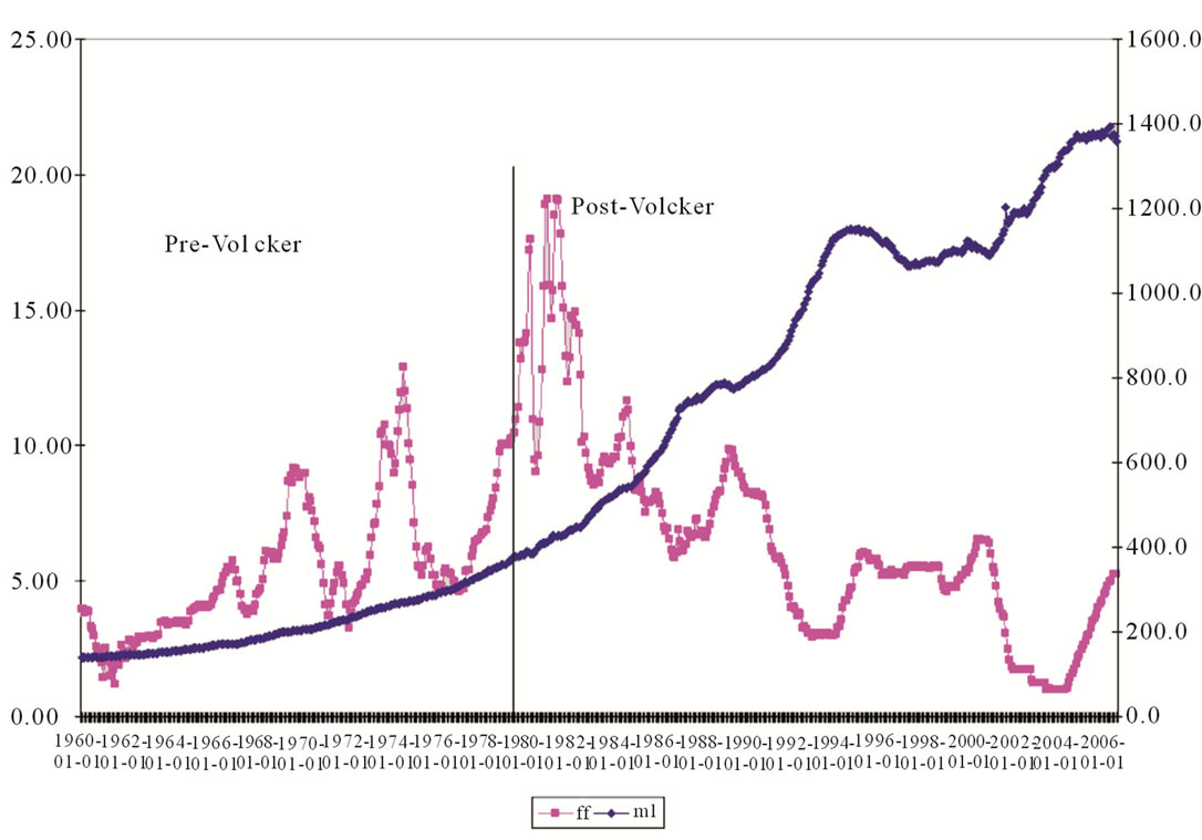
Figure 1. The FF (% per annum) and M1 (in billions of USD).
Larger scale VARs were also estimated, allowing for the reserves market through TR and NBRD. The benchmark 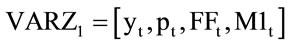 implies that FF rate responds to current innovations in output and prices in a “Taylor rule” fashion: [12]. Money is assumed to respond contemporaneously to the federal funds rate. We do not restrict the VAR model a priori, which is common practice in the price puzzle literature. The augmented model
 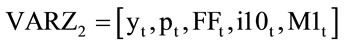 takes into account inflationary expectations and examines 10-year T-Bond interest rates during the “Volcker disinflation” recorded by [13].
4. Results
We apply logarithms to all series, except for interest rates.
The VARs are estimated with 12 lags. Formal serial correlation LM tests on the VAR residuals do not reject the null that no residual correlation exists at lag order h.
Correlation coefficients in Table 1 make clear the distinctive patterns. First, M1 is positively related to FF in the pre-Volcker (0.667) and negatively related to FF in the more recent period (–0.854). The latter would be consistent with an expansionary monetary policy moving the funds rate downwards. Second, interest rates (either the overnight FF rate or the 10-year T-bond) correlate positively (between 0.616 and 0.922) with output and prices in the first subsample but negatively (between –0.703 and –0.904) in the second subsample. Third, prices and commodity prices are strongly correlated, as well as prices and money stock.

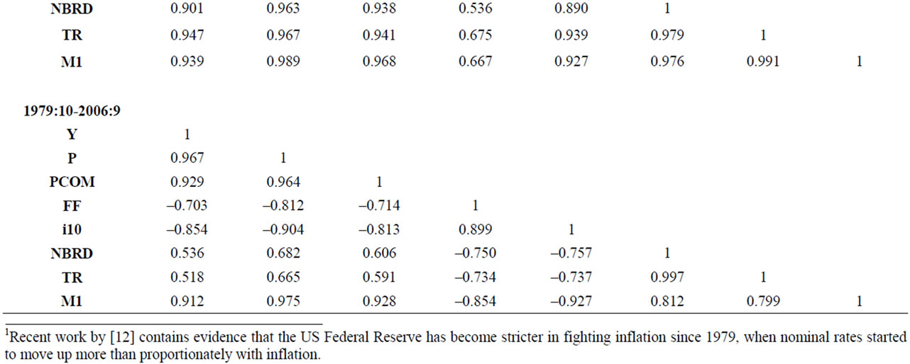
Table 1. Correlation matrices among relevant series for different sample periods.
Figure 2 reports the impulse responses of the benchmark VAR for the pre-Volcker period. For the impulse response functions in Figures 2-5, the responses to Cholesky one standard deviation innovations (with confidence bands) are plotted in the y-axis and time (in months) is plotted in the x-axis. Several findings are worth exploring. First, in the second row, third column, a persistent price puzzle exists for up to 20 months. Innovations in the FF rate have a positive and statistically different from zero effect on the price level. The variance decompositions (VDs) in Table 2 indicate that monetary policy shocks explain 36.5% (1 year) and 31.5% (3 years) of the variance of prices. Second, monetary policy shocks have a negative effect on output at medium horizons. The corresponding VDs indicate that FF shocks explain— after 3 years—almost half (47.3%) of output variance.
Third, federal funds shocks explain about 57.8% of the variance in the FF rate after 3 years of the shock. Under Taylor’s rule, one would expect that a large part of the movements in the funds rate respond to output and prices, which does not happen here. The response in line 3, column 3 of Figure 2 shows a gradually decreasing pattern from the 0.4% response on impact.
Figure 3 displays very different patterns for the postVolcker period. There is no price puzzle now: the shortrun response of the price level to FF shocks is slightly positive. In the long-run, however, increases in FF shocks lead to a fall in the price level, as expected. FF innovations explain only 8.25% of the price variance after 3 years.
In the post-Volcker period output innovations have very strong and persistent effects on FF and on M1. For instance, output shocks lead to positive responses of the FF rate which persist in the medium run for 20 months. VDs indicate that output shocks explain 65.1% of the FF variance after 3 years! Also, increases in output shocks
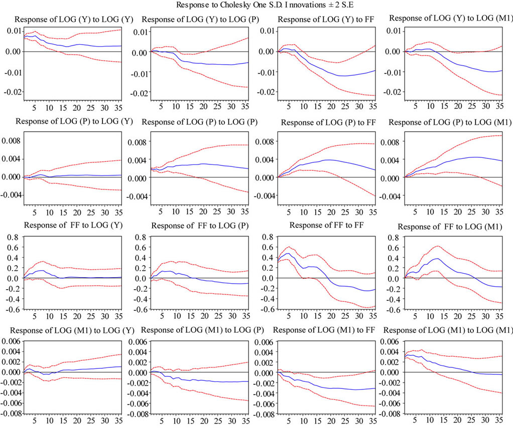
Figure 2. Impulse responses of benchmark VAR: Pre-volcker period, 1960:1 to 1979:9.
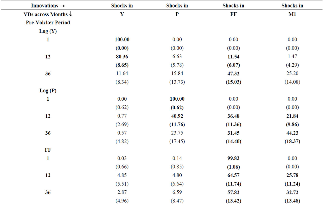
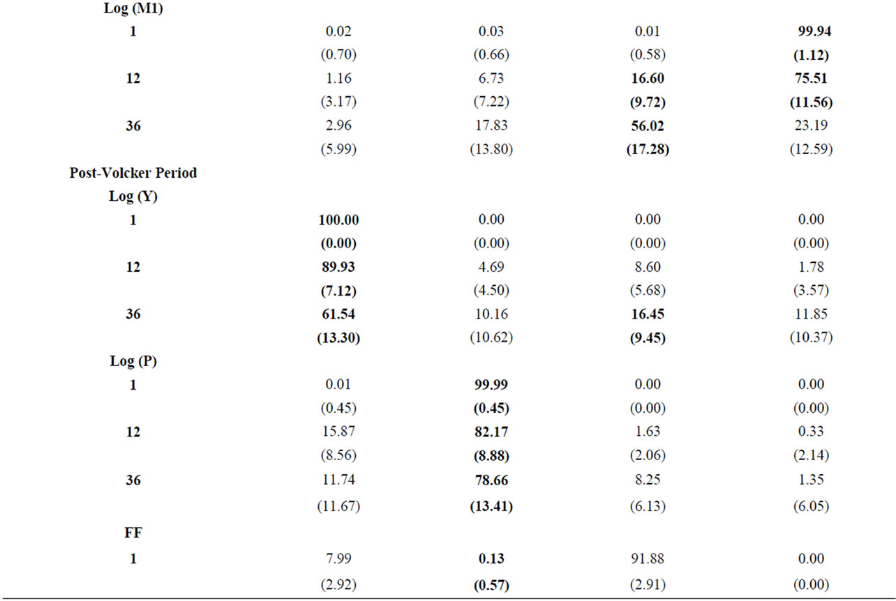

Table 2. Variance decompositions of benchmark VAR Model: X = [Y, P, FF, M1].

Figure 3. Impulse responses of benchmark var: post-volcker period, 1979: 10 to 2006: 9.

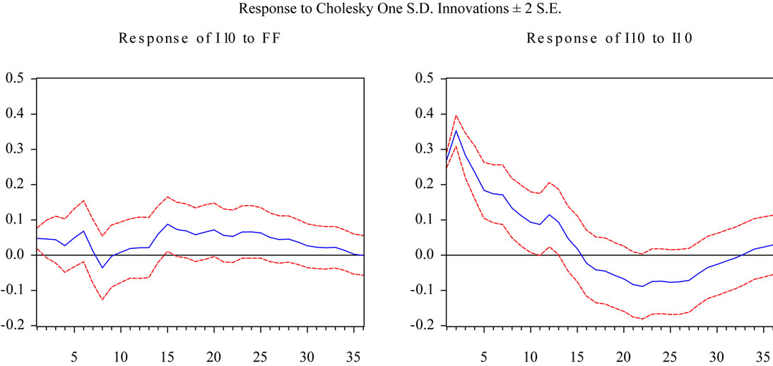
Figure 4. Impulse responses of the long-bond inaugmented VARs; Pre-Volcker (1960:1 to 1979:9) Responses; Post-Volcker (1979:10 to 2006:9) Responses.

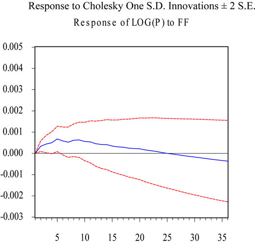
Figure 5. Removing the “monetarist experiment” years; Price Responses to FF from 1979:10 to 2006:9; Price Responses to FF from 1982:11 to 2006:9.
lead to negative responses on the M1 stock, which persist throughout the forecasted horizon. Output shocks explain 64.6% of the variance of M1 after 3 years! In contrast to the earlier period, FF shocks now explain only 28.1% of their own fluctuations after 3 years. There is a much steeper decreasing pattern from the initial 0.6% response.
When the 10-year bond yields are introduced, the augmented VAR for the pre-Volcker period continues to show a persistent price puzzle until the 20th month. However, the response of i10 to shocks in FF is as follows in Figure 4: a positive response at about 0.1% after a one standard deviation FF shock that lasts for about 6 months. This suggests that long-term bonds rise (prices fall) after FF innovations, which is consistent with inflationary expectations remaining high after the contractionary monetary policy shock.
The VDs of i10 explained by FF shocks at 36 months, available upon request, arevery much significant for the pre-Volcker sample with 26.1% (std. deviation of 10.64). Figure 4 for the post-Volcker period shows a close to zero response: long-term bonds respond only on impact to innovations in FF.
Figure 5 initially reproduces Figure 3 with no price puzzle. If one removes the “monetarist experiment” years, however, there is still a price puzzle in the short-run in lower Figure 5, while the long-run has a zero response. This implies that reliance on monetary aggregates in the VAR leads to results in conformity with economic theory and away from the price puzzle.
5. Conclusion
The correlation between money stock and the FF policy instrument has changed remarkably across the two subperiods. Splitting the sample at October of 1979, our VARs do indeed find very contrasting patterns. While the price puzzle is confined to the pre-Volcker period, positive output shocks in the post-Volcker period are followed by price increases, federal funds hikes, and monetary contractions. We interpret our findings under the changing relationship between money and the funds rate across periods. First, the price puzzle is confined to the pre-Volcker period. Second, in the pre-Volcker period the funds rate respond largely to their own shocks, while the post-Volcker period witnesses a larger role for output fluctuations. Third, positive output shocks are more recently followed by price increases, federal funds hikes, and monetary contractions, very much consistent with the “Taylor rule”. Fourth, the “monetarist experiment” of late 1979-1982 reinforces our basic results: the more explicit the reliance on money supply, the less visible the price puzzle becomes.
REFERENCES
- C. Sims, “Interpreting the Macroeconomic Time Series Facts: The Effects of Monetary Policy,” European Economic Review, Vol. 36, No. 5, 1992, pp. 975-1011. doi:10.1016/0014-2921(92)90041-T
- T. Awokuse and J. Yang, “The Informational Role of Commodity Prices in Formulating Monetary Policy: A Reexamination,” Economics Letters, Vol. 79, No. 2, 2003, pp. 219-224. doi:10.1016/S0165-1765(02)00331-2
- M. S. Hanson, “The Price Puzzle Reconsidered,” Journal of Monetary Economics, Vol. 51, No. 7, 2004, pp. 1385-1413. doi:10.1016/j.jmoneco.2003.12.006
- P. Giordani, “An Alternative Explanation of the Price Puzzle,” Journal of Monetary Economics, Vol. 51, No. 6, 2004, pp. 1271-1296. doi:10.1016/j.jmoneco.2003.09.006
- S. Brissimis and N. Magginas, “Forward-Looking Information in VAR Models and the Price Puzzle,” Journal of Monetary Economics, Vol. 53, No. 6, 2006, pp. 1225-1234. doi:10.1016/j.jmoneco.2005.05.014
- B. Mojon, “When Did Systematic Monetary Policy Have an Effect on Inflation?” European Economic Review, Vol. 52, No. 3, 2008, pp. 487-497. doi:10.1016/j.euroecorev.2007.02.007
- D. Krusec, “The ‘Price Puzzle’ in the Monetary Transmission VARs with Long-Run Restrictions,” Economics Letters, Vol. 106, No. 3, 2010, pp. 147-150. doi:10.1016/j.econlet.2009.04.027
- E. Leeper and J. Roush, “Putting ‘M’ Back in Monetary Policy,” Journal of Money, Credit, and Banking, Vol. 35, No. 6, 2003, pp. 1217-1256. doi:10.1353/mcb.2004.0031
- H. Berument and R. Froyen, “Monetary Policy and LongTerm US Interest Rates,” Journal of Macroeconomics, Vol. 28, No. 4, 2006, pp. 737-751. doi:10.1016/j.jmacro.2005.02.004
- B. Bernanke and A. Blinder, “The Federal Funds Rate and the Channels of Monetary Transmission,” American Economic Review, Vol. 82, No. 4, 1992, pp. 901-921.
- L. Christiano, M. Eichenbaum and C. Evans, “The Effects of Monetary Policy Shocks: Evidence from the Flow of Funds,” Review of Economics and Statistics, Vol. 78, No. 1, 1996, pp. 16-34. doi:10.2307/2109845
- R. Clarida, J. Gali and M. Gertler, “Monetary Policy Rules and Macroeconomic Stability: Evidence and Some Theory,” Quarterly Journal of Economics, Vol. 115, No. 1, 2000, pp. 147-180. doi:10.1162/003355300554692
- M. Goodfriend and R. King, “The Incredible Volcker Disinflation,” Journal of Monetary Economics, Vol. 52, No. 5, 2005, pp. 981-1015. doi:10.1016/j.jmoneco.2005.07.001
NOTES
*We would like to thank, without implicating, José Angelo Divino and Walter Enders for helpful comments.
1Recent work by [12] contains evidence that the US Federal Reserve has become stricter in fighting inflation since 1979, when nominal rates started to move up more than proportionately with inflation.