Positioning
Vol.4 No.2(2013), Article ID:31511,9 pages DOI:10.4236/pos.2013.42016
Self-Constructing Neural Network Modeling and Control of an AGV
![]()
Faculty of Mechanical Engineering, University of Tabriz, Tabriz, Iran.
Email: keighobadi@tabrizu.ac.ir
Copyright © 2013 Jafar Keighobadi et al. This is an open access article distributed under the Creative Commons Attribution License, which permits unrestricted use, distribution, and reproduction in any medium, provided the original work is properly cited.
Received February 23rd, 2013; revised March 26th, 2013; accepted April 11th, 2013
Keywords: Wavelet; Neural Networks; Self-Constructing Dynamical Modeling; Trajectory Tracking
ABSTRACT
Tracking precision of pre-planned trajectories is essential for an auto-guided vehicle (AGV). The purpose of this paper is to design a self-constructing wavelet neural network (SCWNN) method for dynamical modeling and control of a 2-DOF AGV. In control systems of AGVs, kinematical models have been preferred in recent research documents. However, in this paper, to enhance the trajectory tracking performance through including the AGV’s inertial effects in the control system, a learned dynamical model is replaced to the kinematical kind. As the base of a control system, the mathematical models are not preferred due to modeling uncertainties and exogenous inputs. Therefore, adaptive dynamic and control models of AGV are proposed using a four-layer SCWNN system comprising of the input, wavelet, product, and output layers. By use of the SCWNN, a robust controller against uncertainties is developed, which yields the perfect convergence of AGV to reference trajectories. Owing to the adaptive structure, the number of nodes in the layers is adjusted in online and thus the computational burden of the neural network methods is decreased. Using software simulations, the tracking performance of the proposed control system is assessed.
1. Introduction
Nowadays, wide range applications of AGVs in industry, transportation, inspection and other fields have increased the importance of the trajectory tracking control of nonholonomic AGVs [1-4]. As the base of path-following controllers, kinematic models of nonholonomic systems have been preferred by most researchers in recent literatures [5]. However, dynamical models though increasing the complexity of control systems are essential due to comprising the vehicle inertial effects as long as its Coriolis, centripetal and linear accelerations in the inputs torques. Furthermore, merely using the dynamical models the input torques to the AGV’s driving wheels could be considered as direct control commands.
In this paper, following kinematic modeling of the generalized AGV whose center of mass is placed out of the center of rotation between two independent driving wheels, the dynamical models of AGV are developed in both Cartesian and polar coordinate systems. Owing to the nonholonomic constraints on AGV’s kinematics, the so-called global dynamical model of AGV includes a coupled constraint equation with two dynamical equations corresponding to 2 DOF of the system. However, the represented dynamical models of AGV by local posture variables don’t include the non-integrable constraints. These kind of dynamical models are more appropriate to design sliding surfaces associate with robust switching controllers [4]. However, as model based controllers require the complete knowledge of the AGV parameters including the inertial matrix, the global dynamical models are superior in the estimation of unknown parameters (see [6,7]).
Furthermore, due to the physical meaning of initial off tracks with respect to global coordinate frames, the control systems based on global dynamical models should be selected when the vehicle is out of the desired path.
Inaccuracies in physical models of AGVs usually degrade the performance of trajectory tracking controllers, therefore, different strategies of solution have been proposed in recent two decades. A nonlinear adaptive controller has been designed based on a dynamical model updated by the online estimation of the plant inertial parameters [1]. Furthermore, robust sliding mode control techniques could be used to accomplish perfect path tracking when there are considerable uncertainties in the mathematical model of systems like an AGV [4,8]. Besides the complicated structure of sliding mode controllers integrated with the plant dynamics, this method is suffered by the chattering phenomenon [9].
Considering the lack of the physical models, the artificial neural networks (ANN) method as a universal function approximation generates a well posed mathematical model with adaptive learning capability. Using a multilayer feed-forward ANN, a combined controller of feedback velocity control and torque control techniques could be developed. However, due to the complicated structures of both the controller and the neural networklearning algorithm, the control system is computationally expensive. Jun has proposed a combined neural network with PID control to take advantage of the simplicity of PID controllers and the powerful capability of learning, adaptability and tackling nonlinearity of neural networks [5,10]. As an important imperfection over most of the developed controllers in the documented research works, the control system merely uses the kinematic equations and therefore, the control commands are limited to the steering angle and forward velocity of the Vehicle. Through developing dynamic based controller, the inertial effects are considered in the imposed torques on the driving wheels as direct control commands to the AGV. In this paper, a four layers back propagation ANN control system for trajectory tracking control of nonholonomic AGVs is designed. A new learning scheme is derived to train the weights of each layer of the neural network by minimizing a criterion prescribed in a quadratic form of the error between desired and followed trajectories by the AGV. A simple torque combined system consisting of a computed torque controller and a neural network controller with parallel structure is presented for trajectory tracking control of nonholonomic AGVs. In the classic NN system, the main drawbacks are undesirable local minima and slow convergence of back-propagation learning. Moreover, the implementation of multiple feed-forward neural networks suffers from the lack of efficient constructive approaches, both for determining parameters of neurons and for choosing network structures. To overcoming the disadvantages of global approximation ANN, the global activation function is substituted with localized wavelet neural networks in the controller [4]. Due to the local properties of wavelets, arbitrary functions can be approximated by the truncated discrete wavelet transform [7].
A self-constructing four-layer wavelet network including input, wavelet, product, and output layers is used to modeling and trajectory tracking control of the vehicle. Using orthogonal wavelet functions as node functions of the network, both the structure and the parameters of the controller are learned in online. In the structure learning process, the degree measure method is used to find the proper wavelet bases and to minimize the number of wavelet bases generated from input space. In parameter learning scheme, the supervisory gradient descent algorithm is used to adjust the shape of wavelet functions and the connection weights of the network. The computed torque SCWN controller based on feedback error learning strategy results in perfect tracking control performance. The rest of the paper is organized as follows.
In Section 2, kinematic and dynamic modeling of AGV is derived. Section 3 is devoted to wavelet neural network modeling of the AGV. Trajectory tracking controllers are represented in Section 4. Software simulation and concluding remarks are presented in Sections 5 and 6, respectively.
2. AGV Kinematics
According to the schematic of AGV in Figure 1, it comprises a plate body carried by two independent driving wheels. The other two caster wheels prevent the vehicle from tipping over as it moves on a plane. Owning to very small inertial moments of the casters, their dynamical effects on the AGV’s motion could be ignored. Per as Figure 1, a is the distance between the center of mass of the vehicle (shown by C) and the connection center of driving wheels. Furthermore, 2l and R denote the length of driving axel and the radius of driving wheels, respectively. The fixed axes of local coordinates, x-y on the vehicle body are centered on point C.
In the dynamical modeling of AGV, the generalized coordinates vector is considered as:
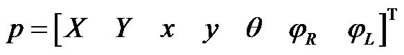 (1)
(1)
where,  and
and  show the position of the AGV’s center of mass in the global coordinate system with axes X-Y; the heading angle between y and Y axes,
  represents the orientation of the AGV in plane motions; and
  are the rotation angles of the right and left driv-
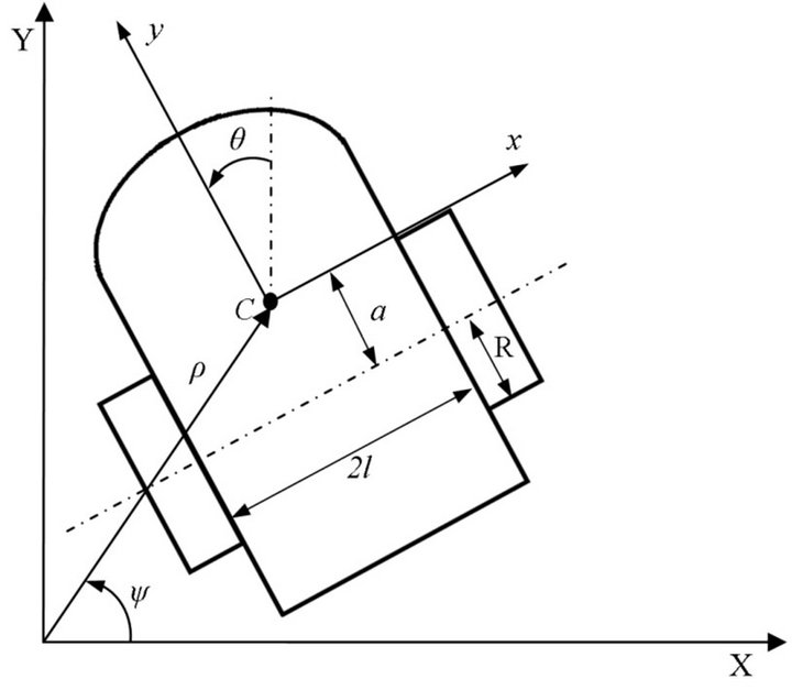
Figure 1. Schematics of AGV.
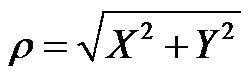
ing wheels, respectively. To explain the AGV’s position in global polar coordinates, the components 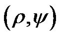 could also be used.
The assumption of pure rolling and not slipping motion of driving wheels leads to a non-integrable constraint in the kinematical model of the nonholonomic vehicles. Therefore, the AGV’s posture could be determined completely using at least three generalized coordinates though its dynamical model comprises only two differential equations.
Considering the AGV kinematics, the following holonomic constraints are valid for movements on non-sliding and smooth surfaces.
 (2)
(2)
 (3)
(3)
 (4)
(4)
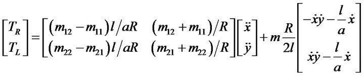
Transforming the local velocity components of AGV to the global components results in the nonholonomic constraints as:
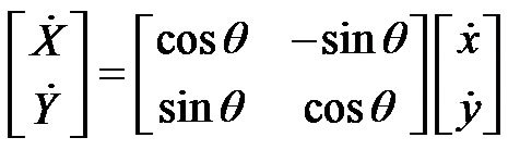 (5)
(5)
These constraints could be rewritten using (1) through (4) to obtain direct transformation matrix between the global velocity components and the local translationalrotational velocity components as:
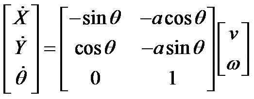 (6)
(6)
where, the local velocity components  and
and  stand for the linear forward velocity of AGV and its angular velocity around the vertical axis, respectively.
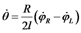
Using the posture variables of polar coordinate system,
 and
and 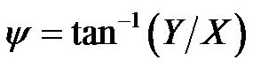 in (6), the kinematical model of AGV in polar coordinates is obtained as follows.
 (7)
(7)
The considered distance between the centers of rotation and mass of the AGV,  leads to an enlarged application range of the proposed methods to different kind of industrial, service and entertainment vehicles.
Owing to excluding the inertial effects, the designed controllers based on the kinematical models (2) through (7) may not be very satisfied in real world at least for mechanical engineers. Furthermore, the dynamical models of AGV should be used as the base of control systems to obtain the input torques to AGV as direct control commands.
3. Dynamic Modelling of AGV
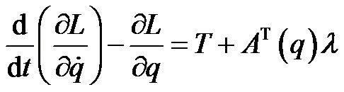
In the dynamical models, the applied torques to the driving wheels would be obtained as terms of the vehicle accelerations, velocities, and posture variables as well as the inertial parameters. In this paper, the well-known Lagrange’s method is used to determine the dynamical equations of motion as:
 (8)
(8)
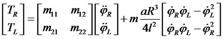
where,  is a Lagrange multiplier;
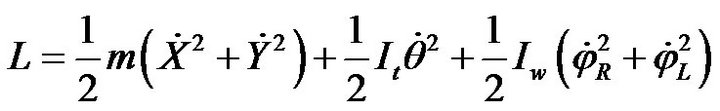
  is given by the nonholonomic constraints; and T is the control torque vector with components, TR and TL which are generated by separate actuator motors of the right and left driving wheels, respectively. Now the following Lagrangian could be considered for the AGV dynamic modeling [1].
 (9)
(9)
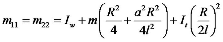
where, m is the total mass of the vehicle;  is the AGV’s moment of inertia around the normal axis of X-Y plane crossing through the point C; and
  denotes the inertia moment of driving wheels. Applying (9) in (8) and using the kinematical constraints (2) through (5) gives:
 (10)
(10)
 (11)
(11)
 (12)
(12)
 (13)
(13)
 (14)
(14)
 (15)
(15)
 (16)
(16)
As represented by Hu and Huo [11], many nonholonomic mechanical systems could be described by Equation (10) in which in general form,  and
and  are the generalized configuration and the control input vectors, respectively;
  is the constraint force vector;
  is a positive definite matrix;
  is the term which includes centripetal and Coriolis forces;
  is a
is a  full rank transformation input matrix;
  is a
is a  full rank matrix associated with the constraints.
In order to achieve an applicable model for control purposes, the constraint force vector,  should be eliminated from (10). Depending on using which set of kinematical equations, four different dynamical models are presented in this paper. Using constraints (2) through (5), the following so called local dynamic model is obtained.
 (17)
(17)
 (18)
(18)
 (19)
(19)
Using (2) and (3) in (17) to replacing  by
by  results in another so-called local dynamical model of AGV as:
 (20)
(20)
Using local dynamical models as the base of path following control systems results in uncompensated initial position off tracks though the tracked orientation trajectory by the AGV becomes accurate [4]. To overcome this difficulty, two dynamical models of AGV are developed using global posture variables. Therefore, using constraints (5) to replacing the local velocity and acceleration components in (20) by corresponding global kinds results as:
 (21)
(21)
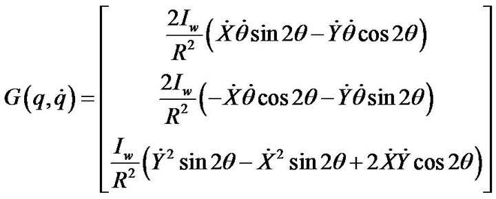
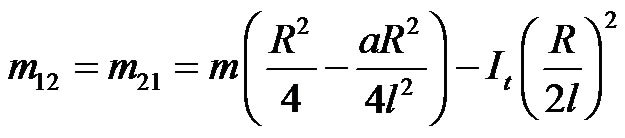
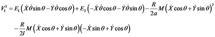
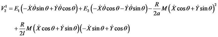
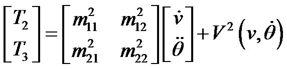
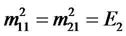
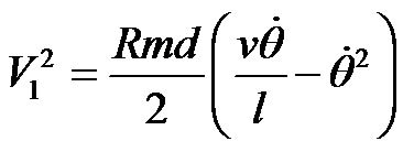
The elements of inertial matrix and nonlinear vector,  associated with the global dynamical model (21) are obtained as:
 (22)
(22)
 (23)
(23)
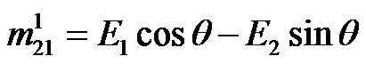 (24)
(24)
 (25)
(25)
 (26)
(26)
 (27)
(27)
where:
 (28)
(28)
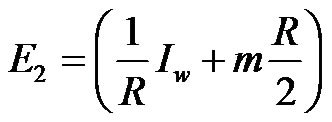 (29)
(29)
By use of kinematical model (6),  and
and  could be written in terms of
  and
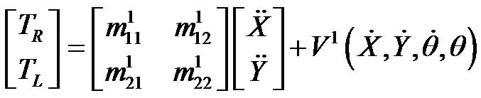
and . Hence, (21) is changed to the second dynamical model in global coordinate system as:
 (30)
(30)
 (31)
(31)
 (32)
(32)
 (33)
(33)
 (34)
(34)
Unlike the model (21), the represented model (30) is simple and its inertial matrix doesn’t include the posture variables of AGV. Therefore, this new dynamical model (30) is not affected by probable measurement noises of orientation variable, .
.
4. Wavelet Neural Network (WNN)
As the base of a control system, the mathematical models are not preferred due to modeling uncertainties and exogenous inputs affecting real systems. In this section dynamical modeling of the AGV is considered as a self-constructing wavelet neural network (SCWNN) system. As shown in block diagram of Figure 2, the SCWNN receives a vector of desired reference position, velocity and orientation trajectories,  that should be tracked by the AGV. Through the learned SCWNN, the input torque vector, T which should be imposed on the driving wheels of the AGV is generated. Therefore, the AGV will track the desired position and orientation posture variables by applying the intelligently produced torque vector, T. The structure of the designed wavelet neural network (WNN) model is shown in Figure 3.
The proposed SCWNN has a four-layer structure comprising of the input layer, wavelet layer, product layer, and output layer. The input data to the first layer of the network is a n-dimensional vector of posture variables as,  which is normalized into the interval
 . The activation functions of wavelet nodes in the second layer are derived from the mother wavelet,
  with a dilation, d and a translation t as:
 . The mother wavelet is selected in such a way that it constitutes an orthonormal basis in
 . The derivation of a differentiable Mexican-hat function is considered as a mother wavelet herein [8],
 (35)
(35)
where  stands for 2-norm of vector. Consequently, the activation function of the j-th wavelet node connected with the i-th input data is represented as:
where, n is the number of input-dimensions and m is the number of the wavelets. The wavelet functions (35) with various dilations and translations are presented in Figure 4. Then, each wavelet in the product layer is labeled P, i.e., the product of the jth multidimensional wavelet with n input dimensions , can be defined as
 (37)
(37)
According to the theory of multi-resolution analysis (MRA), see [8], any  can be regarded as a linear combination of wavelets at different resolution levels. For this reason, the function
  is expressed as
 (38)
(38)
If  is used as a nonlinear transformation function of hidden nodes and weight vectors and
  defines the connection weights, then Equation (38) can be considered the functional expression of the SCWN modeling function Y.
4.1. Self-Constructing Learning Algorithm
In this section, the degree measure method and the well-known back propagation (BP) algorithm are used concurrently for constructing and adjusting the SCWN algorithm. The degree measure method is used to determine the number of wavelet bases in the wavelet layer and the product layer. Furthermore, the BP algorithm is used to adjust the parameters of the wavelet bases and connection weights. At the initial time, the SCWN system does not comprise any wavelet bases. Therefore, the first task is to decide when a new wavelet base should be generated. The partition-based clustering techniques are used to perform cluster analysis in a data set. For each incoming pattern , the firing strength of a wavelet base can be regarded as the degree of the incoming pattern belonging to the corresponding wavelet base. An input datum
 , with a higher firing strength means that its spatial location is nearer to the center of the wavelet
|
|
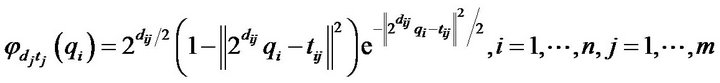
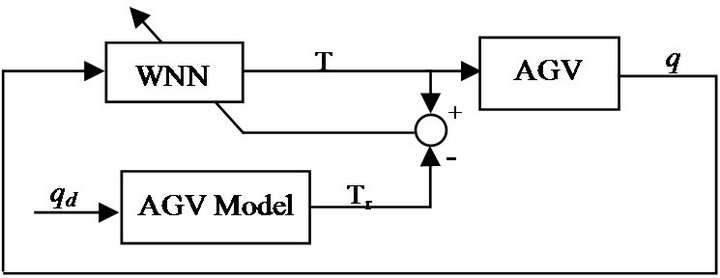
Figure 2. Block diagram of SCWNN modeling system.

Figure 3. Structure of wavelet neural network.
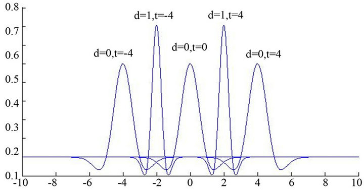
Figure 4. Wavelet functions of (35) with various dilations and translations.
base , than those with smaller firing strength. Based on this concept, the firing strength obtained from Equation (37) in the product layer can be used as the degree measure.
 (39)
(39)
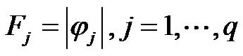
where,  is the number of existing wavelet bases and
 , is the absolute value of
 . According to the degree measure, the criterion of a new wavelet base generated for new incoming data is described in the block diagram of Figure 5.
In Figure 5  is a prespecified threshold that should decay during the learning process, limiting the size of the SCWN model and
  are new wavelet’s parameters according as regarded Initially, there are no wavelet bases in the SCWN controller. The first task is to decide when a new wavelet base is generated. We adopt partition-based clustering techniques to perform cluster analysis in a data set. For each incoming pattern
 , the firing strength of a wavelet base can be regarded as the degree of the incoming pattern belonging to the corresponding wavelet base. An input datum
  with a higher firing strength means that its spatial location is nearer to the center of the wavelet base
  than those with smaller firing strength.
  is defined as,
  where, n is the number of input variables.
After the network structure has been adjusted according to the current training pattern, the network then enters the second learning step to adjust the parameters of the wavelet base and the connection weight ( and
and ) with the same training pattern. The parameterlearning algorithm is based on a set of input/output pairs
 . If the error function is
 (40)
(40)
where  is the model output and
  is the desired output, then the cost function E can be defined as
 (41)
(41)
and can be minimized by all adjustable parameters using an iterative computational scheme. Assuming that W is the adjustable parameter in the wavelet layer and the output layer, the general learning rule used is
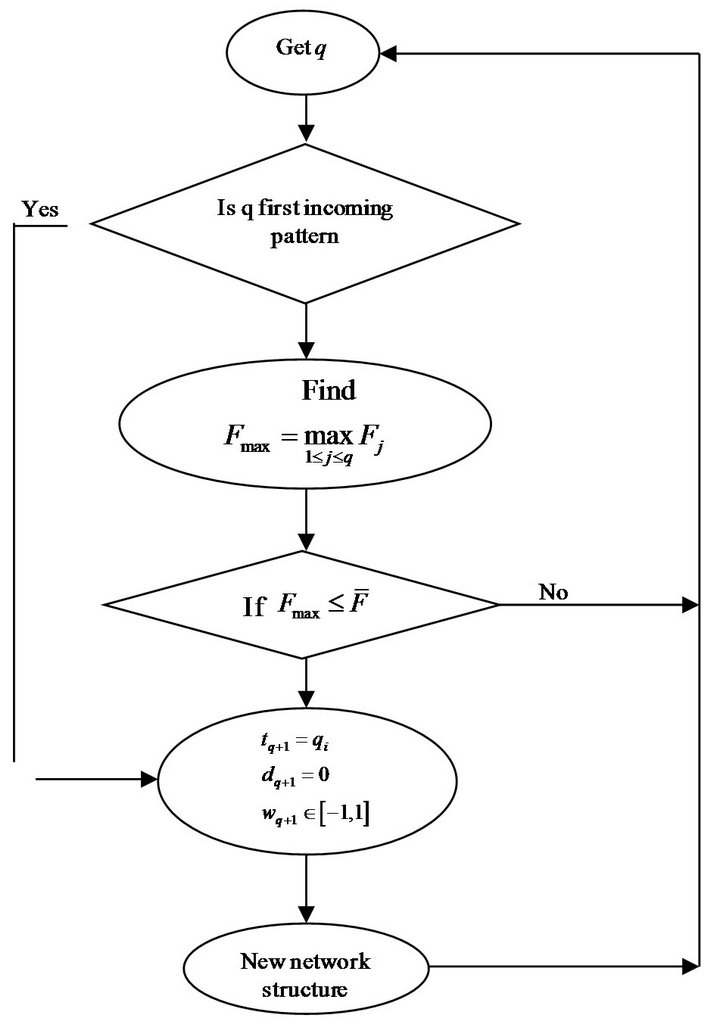
Figure 5. Block diagram for generation of new wavelets in SCWN.
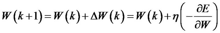 (42)
(42)
where  and
and  represent the learning rate and the iteration number, respectively. The gradient of the cost function
  in Equation (41) with respect to the vector of arbitrarily adjustable parameter
  is defined as
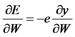 (43)
(43)
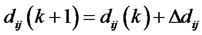
With the above equation defined, we can infer that the free parameters adjusted in the SCWN are as follows. The connection weight of the output layer is updated by
 (44)
(44)
Similarly, the updated laws of  and
and  are shown as follows:
 (45)
(45)
 (46)
(46)
where
4.2. Wavelet Neural Network Control of AGV
Neural networks have known as an attractive method to model the complex non-linear systems due to its inherent ability to approximate arbitrary continuous functions. During the 1980’s and the early 1990’s, conclusive proofs were given by numerous authors that feed-forward neural networks with one hidden layer are capable of approximating any continuous function on a compact set in a very precise and satisfactory sense [12]. Recently, wavelet decomposition method has been used as a new powerful tool for function approximation in a manner that readily reveals properties of the arbitrary L2 function (energy-finite and continuous or discontinuous) [13]. Combination of wavelets and neural networks methods results in wavelet neural network models with efficient constructive approach. Besides precise approximation of arbitrary L2 functions, the wavelet neural networks could result in a convex cost index for which simple iterative solutions such as gradient descent rules are justifiable and are not in danger of being trapped in local minima when choosing the orthogonal wavelets as the activation functions in the nodes [8]. In this paper, the WNN technique is used as the inverse dynamic model of the AGV to generate sufficient robustness against modeling uncertainties and exogenous disturbances. Considering the proposed dynamical model (17), the input variables to the WNN system are supposed as follow.
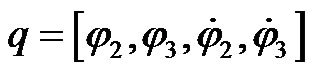 (49)
(49)
Owing to the fact that the nonholonomic AGV is a 2 DOF dynamic system, two separate WNN systems are used to approximate the input torque of every driving wheels of the AGV. In this way, two control actions for trajectory tracking control of the AGV,  and
and  are computed by the right and left WNN as shown in Figure 6.
5. Simulation Results
Using simulations, the effects of the proposed wavelet neural network controller on the convergence of AGV to reference trajectories are evaluated. Therefore, the following example trajectories are used to produce the reference position and orientation angle of the AGV.
 (50)
(50)
 (51)
(51)
 (52)
(52)
The simulation of the WNN controller results in a perfect trajectory tracking performance of the AGV. The comparison of tracked X, Y and also the complete circular path of the AGV with the reference values are shown in Figures 7-9, respectively. From these figures, the tracking convergence of AGV along both X and Y trajectories is very fast.
6. Conclusion
An intelligent wavelet neural networks modelling and control method of an AGV has been proposed. Owing to the self-constructing nature of the proposed WNNT, the number of nodes in the layers of the WNNT system is adjusted automatically. Therefore, the proposed method
|
|
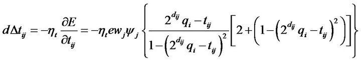
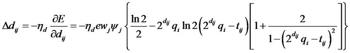

Figure 6. block diagram of AGV control system with inverse dynamic.

Figure 7. Tracking of AGV along X axes.
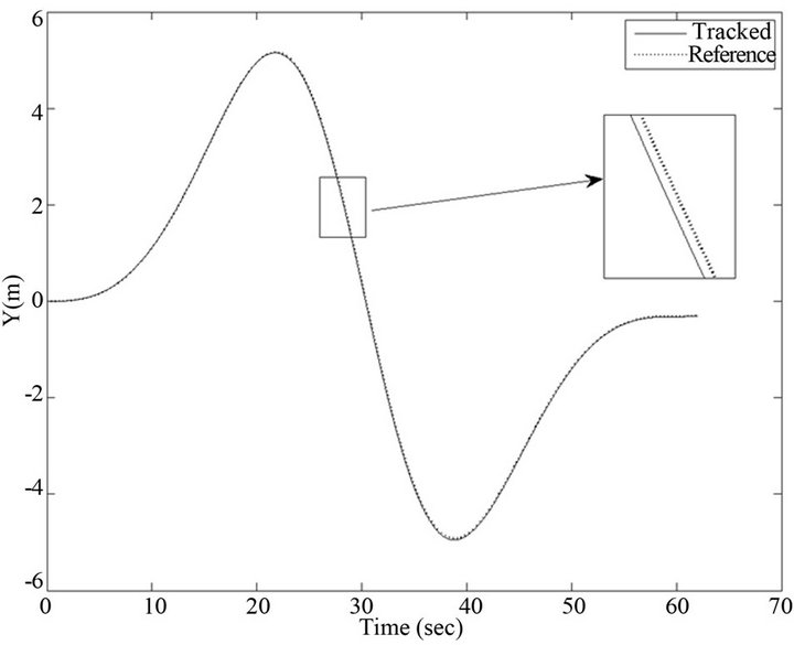
Figure 8. Tracking of AGV along Y axis.
does not require the fixed number of nodes and thereby the computation cost is reduced. Unlike kinematic models, the SCWNN dynamic model of the AGV results in considering the inertial, Coriolis and centripetal accelera-

Figure 9. Tracking of AGV on XY plane.
tions in the trajectory tracking control of the vehicle. According to simulation results, the WNNT control system yields a perfect trajectory tracking of the AGV.
REFERENCES
- J. Keighobadi, M. B. Menhaj and M. Kabganian, “Feedback Linearization and Fuzzy Controllers for Trajectory Tracking of Wheeled Mobile Robots,” Kybernetes, Vol. 39, No. 1, 2010, pp. 83-106. doi:10.1108/03684921011021291
- J. Keighobadi, “Fuzzy Calibration of a Magnetic Compass for Vehicular Applications,” Mechanical Systems and Signal Processing, Vol. 25, No. 6, 2011, pp. 1973-1987. doi:10.1016/j.ymssp.2010.11.005
- J. Keighobadi, M. J. Yazdanpanah and M. Kabganian, “An Enhanced Fuzzy H∞ Estimator Applied to Low-Cost Attitude-Heading Reference System,” Kybernetes, Vol. 40, No. 1, 2011, pp. 300-326. doi:10.1108/03684921111118068
- J. Keighobadi and M. B. Menhaj, “From Nonlinear to Fuzzy Approaches in Trajectory Tracking Control of Wheeled Mobile Robots,” Asian Journal of Control, Vol. 14, No. 4, 2012, pp. 960-973. doi:10.1002/asjc.480
- Y. Jun, “Adaptive Control of Nonlinear PID-Based Analog Neural Networks for a Nonholonomic Mobile Robot,” Neuro-Computing, Vol. 71, No. 7-9, 2008, pp. 1561-1565. doi:10.1016/j.neucom.2007.04.014
- Q. Zhang, “Using Wavelet Networks in Nonparametric Estimation,” IEEE Transactions on Neural Networks, Vol. 8, No. 2, 1998, pp. 227-236. doi:10.1109/72.557660
- J. Q. Guo, B. Y. Hai and D. X. Ai, “An Online Self-Constructing Wavelet Fuzzy Neural Network for Machine Condition Monitoring,” Proceeding of the 4th International Conference on Machine Learning and Cybernetics, Guangzhou, 18-21 August 2005, pp. 18-21.
- C. J. Lin, “Nonlinear Systems Control Using Self-Constructing Wavelet Networks,” Applied Soft Computing, Vol. 9, No. 1, 2009, pp. 71-79. doi:10.1016/j.asoc.2008.03.014
- J. Keighobadi and Y. Mohamadi, “Fuzzy Robust Trajectory Tracking Control of WMRs,” In: S. I. Ao, O. Castillo, and X. Huang, Eds., Intelligent Control and Innovative Computing, Springer, Singapore, 2012, pp. 77-90. doi:10.1007/978-1-4614-1695-1_7
- L. Gaviphat, “Adaptive Self-Tuning Neuro Wavelet Network Controllers,” Ph.D. Thesis, Electrical Engineering Department, Blackburg, 1997.
- M. Y. Hu and W. Huo, “Robust and Adaptive Control of Nonholonomic Mechanical Systems with Application to Mobile Robots,” In: T. P. Leung and H. S. Qin, Eds., Advanced Topics in Nonlinear Control Systems, 2001, pp. 161-192.
- M. R. Sanner and J. J. E. Slotine, “Structureally Dynamic Wavelet Networks for Adaptive Control of Robotic Systems,” International Journal of Control, Vol. 70, No. 3, 1998, pp. 405-421. doi:10.1080/002071798222307
- F. J. Lin, R. J. Wai and M. P. Chen, “Wavelet Neural Network Control for Linear Ultrasonic Motor Drive via Adaptive Sliding-Mode Technique,” IEEE Transactions on Ultrasonics, Ferroelectrics and Frequency Control, Vol. 50, No. 6, 2003, pp. 686-698. doi:10.1109/TUFFC.2003.1209556