Positioning
Vol.4 No.1(2013), Article ID:28372,16 pages DOI:10.4236/pos.2013.41004
Mobile Robot Indoor Autonomous Navigation with Position Estimation Using RF Signal Triangulation
![]()
1Department of Electrical Engineering, State University of Londrina (UEL), Londrina, Brazil; 2Mechanical Engineering Faculty, State University of Campinas (UNICAMP), Campinas, Brazil.
Email: leonimer@uel.br
Received November 2nd, 2012; revised December 3rd, 2012; accepted December 15th, 2012
Keywords: Mobile Robotic Systems; Path Planning; Mobile Robot Autonomous Navigation; Pose Estimation
ABSTRACT
In the mobile robotic systems a precise estimate of the robot pose (Cartesian [x y] position plus orientation angle theta) with the intention of the path planning optimization is essential for the correct performance, on the part of the robots, for tasks that are destined to it, especially when intention is for mobile robot autonomous navigation. This work uses a ToF (Time-of-Flight) of the RF digital signal interacting with beacons for computational triangulation in the way to provide a pose estimative at bi-dimensional indoor environment, where GPS system is out of range. It’s a new technology utilization making good use of old ultrasonic ToF methodology that takes advantage of high performance multicore DSP processors to calculate ToF of the order about ns. Sensors data like odometry, compass and the result of triangulartion Cartesian estimative, are fused in a Kalman filter in the way to perform optimal estimation and correct robot pose. A mobile robot platform with differential drive and nonholonomic constraints is used as base for state space, plants and measurements models that are used in the simulations and for validation the experiments.
1. Introduction
The mobile robotics is a research area that deals with the control of autonomous vehicles or half-autonomous ones. In mobile robotics area one of the most challenger topic is keep in the problems related with the operation (locomotion) in complex environments of wide scale, that if modify dynamically, composites in such a way of static obstacles as of mobile obstacles. To operate in this type of environment the robot must be capable to acquire and to use knowledge on the environment, estimate a inside environment position, to have the ability to recognize obstacles, and to answer in real time for the situations that can occur in this environment. Moreover, all these functionalities must operate together. The tasks to perceive the environment, to auto-locate in the environment, and to move across the environment are fundamental problems in the study of the autonomous mobile robots [1].
The planning of trajectory for the mobile robots, and consequently its better estimative of positioning, is reason of intense scientific inquiry. A good path planning of trajectory is fundamental for optimization of the interrelation between the environment and the mobile robot. A great diversity of techniques based in different physical principles exists and different algorithms for the localization and the planning of the best possible trajectory [2].
The localization in structuralized environment is helped, in general, by external elements that are called landmarks (or markers). Landmarks can be active or passive, natural or artificial. It is possible to use natural landmarks that already existing in the environment for the localization. Another possibility is to add intentionally to the environment artificial landmarks for guide the localization of the robot. Active landmarks, also called beacons, are typically transmitters that emit unique signals and are placed about the environment [3].
This work uses a ToF of the RF digital signal interacting with RF beacons for computational triangulation in the way to provide a pose estimative at bi-dimensional indoor environment. It’s a new technology utilization making good use of old ultrasonic ToF methodology that takes advantage of high performance multicore DSP processors to calculate ToF of the order about ns. Sensors data like odometry, compass and the result of traingulation Cartesian estimative, are fused in a Kalman filter in the way to perform optimal estimation and correct robot pose. A mobile robot platform with differential drive and nonholonomic constraints is used as base for state space, plants and measurements models that are used in the simulations and for validation the experiments [4].
First are presented the kinematic and dynamic model used for simulations and for implement a control strategy in order to best performance of robot embedded control system. After are presented the control architecture system, including supervisory, communication and embedded robot control system. It’s important to situate the reader in the context of our experiments a researching. Then, are presented the trajectory embedded control and after the technique adopted here for triangulation with digital RF signal beacons. After all, are shown the data fusion using Kalman Filter, for best robot pose estimative and rout corrections. At the end of this paper, we present some initial experimental results and a few conclusions.
2. Kinematics for Mobile Robots with Differential Traction
This work focus on the study of the mobile robot platform, with differential driving wheels mounted on the same axis and a free castor front wheel, whose prototype used to validate the proposal system, is depicted in Figures 1 and 20 which illustrate the elements of the platform.
Assuming that the robot is in one certain point  directed for a position throughout a line making an angle theta with x axis, as illustrated in the Figure 2.
Through the manipulation the control parameters ve and vd, the robot can be lead at different positionings. The determination of the possible positionings to be reached, once given the control parameters, is known as direct kinematics problem for the robot. As illustrated in the Figure 2, in which the robot is located in position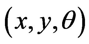 , we have for the trigonometrical relations of the system,
 (1)
(1)
where ICC is the robot instantaneous curvature center.
As ve and vd are time functions and if the robot is in the pose  in the time t, and if the left and right wheel has ground contact speed ve and vd respectively,

Figure 1. Illustrative mobile robot platform and elements.

Figure 2. Direct kinematics for differential traction in mobile robots.
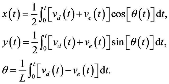
then, in the time  the position of the robot is given by
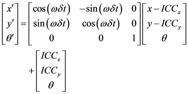 (2)
(2)
The Equation (2) describes the motion of a robot rotating a distance R about its ICC with an angular velocity given by ω [2]. Different classes of robots will provide different expressions for R and ω [5].
The forward kinematics problem is solved by integrating Equation (2) from some initial condition , it is possible to compute where the robot will be at any time t based on the control parameters
  and
and . For the special case of a differential drive vehicle, it is given by Equation (3).
 (3)
(3)
Inverse Kinematics for Differential Drive Robots
Equation (3) describes a constraint on the robot velocity that cannot be integrated into a positional constraint. This is known as a nonholonomic constraint and it is in general very difficult to solve, although solutions are straightforward for limited classes of the control functions  and
and  [6]. For example, if it is assummed that
  and
and , then Equation (3) yields into Equation (4):
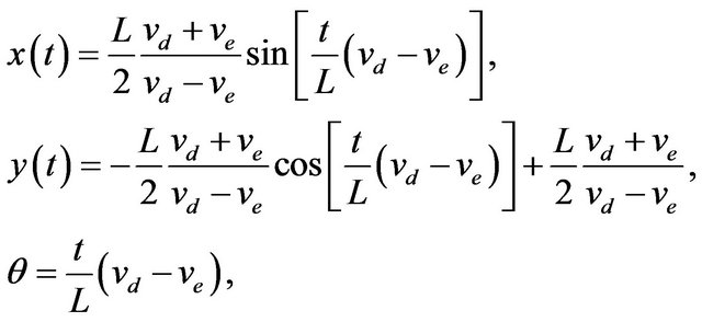 (4)
(4)
where . Given a goal time t and goal position
 . The Equation (4) solves for vd and ve but does not provide a solution for independent control of θ. There are, in fact, infinity solutions for vd and ve from Equation (4), but all correspond to the robot moving about the same circle that passes through (0, 0) at t = 0 and
  at t = t; however, the robot goes around the circle different numbers of times and in different directions.
3. The Control Architecture System
The control architecture system can be visualized at a logical level in the blocks diagram in Figure 3.
The system was divided into three control levels, organized in the form of different degrees of control strategies. The levels can be described as:
• Supervisory control level: This represents a high level of control. In this level it was possible to carry out the supervision of one or more mobile robots, through the execution of global control strategies.
• Local onboard control level: In this level control was processed by the mobile robot embedded software implemented in a multicore DSP processor. The control strategies allowed decision making to be done at a local level, with occasional corrections from the
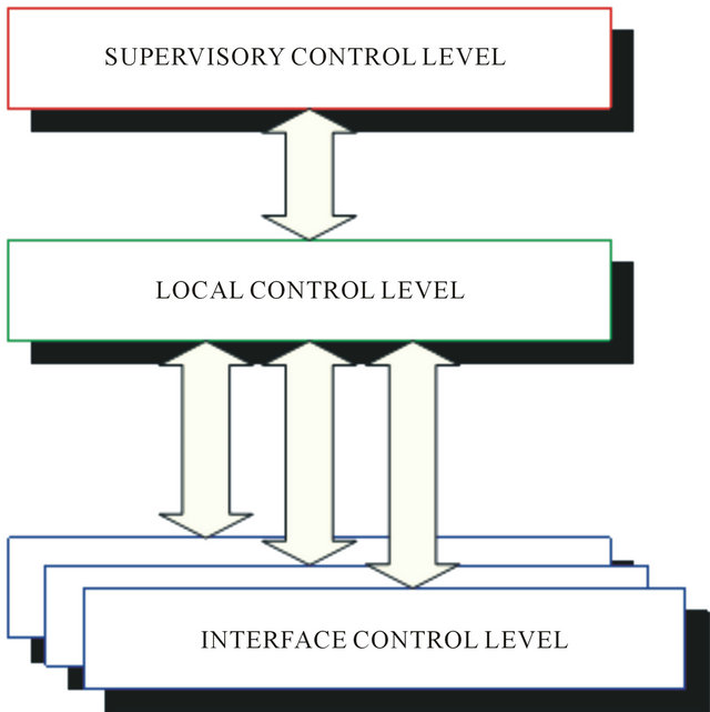
Figure 3. Illustrative mobile robot platform and elements.
supervisory control level. Without communication with the supervisory control level, the mobile robot just carried out actions based on obtained sensor data and on information previously stored in its memory.
• Interface control level: This was restricted to strategies of control associated with the interfaces of the sensor and actuators. The strategies in this level were implemented in hardware, through FPGA (FieldProgrammable Gate Array) device.
Figure 4 depicts the control architecture with more details, with the levels controls implemented on the mobile robot platform.
Architecture, from the point of view of the mobile robot, was organized into several independent blocks, connected through the local bus that is composed by data, address and control bus (Figure 5). A master block manager operates several slave blocks. Blocks associated with the interfaces of sensors and actuators, communication and auxiliary memories were subjected to direct control from the block manager. The advantage of using a common bus was the facility to expand the system. Inside the limitations of resources, it was possible to add new blocks, allowing an adapted configuration of the robot for each task.

Figure 4. Mobile Robot control architecture.
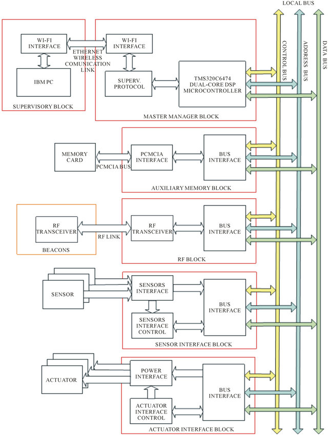
Figure 5. Hardware architecture block diagram of the proposed system.
Control Architecture Blocks Description
Supervisory control block: It’s the high level of control. In this block is managed the supervision of one or more mobile robots, through the execution of global control strategies. Is implemented in an IBM PC platform and is connected with the local control level, in the mobile robot, through Ethernet wireless WI-FI link. This protocol uses IEEE 802.11a standard for wireless TCP/IP LAN communication. It guarantees up to 11 Mbps in the 2.4 GHz band and requires fewer access points for coverage of large areas. Offers high-speed access to data at up to 100 meters from base station. 14 channels available in the 2.4 GHz band guarantee the expansibility of the system with the implementation of control strategies of multiple robots.
Master manager block: It’s responsible for the treatment of all the information received from other blocks, for the generation of the trajectory profile for the local control blocks and for the communication with the external world. In communication with the master manager block, through a serial interface, a commercial platform was used, which implemented external communication using an Ethernet WI-FI wireless protocol. The robot was seen as a TCP/IP LAN point in a communication net, allowing remote supervision through supervisory level. It’s implemented with Texas Instrument TMS320C6474 multicore digital signal processor, a 1.2 GHz device delivering up to 10,000 million instructions per second (MIPs) with highest performing.
Sensor interface block: Is responsible for the sensor acquisition and for the treatment of this information in digital words, to be sent to the master manager block. The implementation of that interface through FPGA allowed the integration of information from sensors (sensor fusion) locally, reducing manager block demand for processing. In same way, they allowed new programming of sensor hardware during robot operation, increasing sensor treatment flexibility.
Actuator interface block: This block carried out speed control or position control of the motors responsible for the traction of the mobile robot. The reference signals were supplied through bus communication in the form of digital words. Derived information from the sensor was also used in the controller implemented in FPGA. Due to integration capacity of enormous hardware volume, FPGA was appropriate to implement state machines, reducing the need for block manager processing. Besides the advantage of the integration of the hardware resources, FPGA facilitated the implementation and debugging. The possibility of modifying FPGA programming allowed, for example, changes in control strategies of the actuators, adapting them to the required tasks.
Auxiliary memory block: This stored the information of the sensor, and operated as a library for possible control strategies of sensors and actuators. Apart from this, it came with an option for operation registration, allowing a register of errors. The best option was an interface PCMCIA, because this interface is easily accessible on the market, and being a well adapted for applications in mobile robots, due to low consumption, little weight, small dimensions, high storage capacity and good immunity to mechanical vibrations.
RF beacons communication block: It allowed the establishment of a bi-directional radio link for beacons data communication. The objective, at the first moment, is establish communication with all beacons in the environment, not at same time, but one by one, recognizing the number of active beacons and their respective codes. At second moment, this RF communication block sends a determinate code and receive back the same code, transmitted from respective beacon. The RF ToF is calculated by DSP processor. To implement this block was used a low power UHF data transceiver module BiM-433-40.
4. Trajectory Embedded Control
Figure 6 illustrates an example of an environment with some obstacles where the robot must navigate. In this environment, the robot is located initially in the P1 point and the objective is to reach the P4 point. The supervisory generating system of initial Cartesian points, must then supply to the module of embedded trajectory generation, the Cartesian points P1, P2, P3 and P4, which are the main points of the traced route. Figure 7 presents a general vision of the trajectory generator system.

Figure 6. Example of an environment with some obstacles where the robot must navigate.
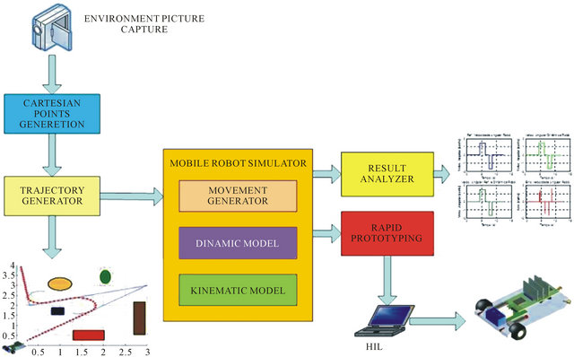
Figure 7. General vision of the trajectory generator system.
The use of the system begins with the capitation of main points for generation of the mobile robot trajectory. The idea is to use a system of photographic video camera that catches the image of the environment where the mobile robot will navigate. This initial system must be capable to identify the obstacles of the environment and to generate a matrix with some strategically points that will serve of input for the system of embedded trajectory generation [7]. The mobile robot embedded control system receives initially, through the supervisory system, a trajectory to be executed. These data are loaded in the robot memory that is sent to the module of trajectory generation. At a time the robot starts to execute the trajectory, the dynamic data are returned to the embedded controller, who, with the measurements and sensing, makes the comparisons and due corrections in the trajectory.
The trajectory embedded control system of the mobile robot is formed by three main blocks. The first one is called movements generation block.
The second is the block of the controller and dynamic model of the mobile robot. Third is the block of the kinematic model. Figure 8 illustrates the mobile robot control strategy implemented into Matlab Simulink blocks and then loaded in the embedded memory of the DSP processor by HIL (hardware-in-the-loop) technique.
The mobile robot embedded control is implemented with kinematic model presented at Section 2, the dynamic model for axles control and the movement generator modules. Figure 9 illustrates the blocks diagram representing those modules.
The input system variables are:
• ∆t is the period between one pose point and another.
• TJref, is the reference trajectory matrix given by supervisory control block with all the trajectory dots pose coordinates .
.
• Vref, is the robot linear velocity dynamics informed by supervisory control block so that robot can accomplish one particular trajectory.
The embedded system output variables are:
• TJdin, that is the robot dynamic trajectory matrix, given in Cartesian coordinate format.
• Vdin, is the dynamic linear velocity of the robot.
• Rc, is the mobile robot ICC.
• θ, is the orientation angle.
• ω, is the angular velocity vector.
5. Position Estimation with RF Signal ToF
The communication system between the mobile robot and the beacons is follow described. The mobile robot and each one of the beacons, have a module of control and reception of the address codes and a module of transmission. The communication protocol between the
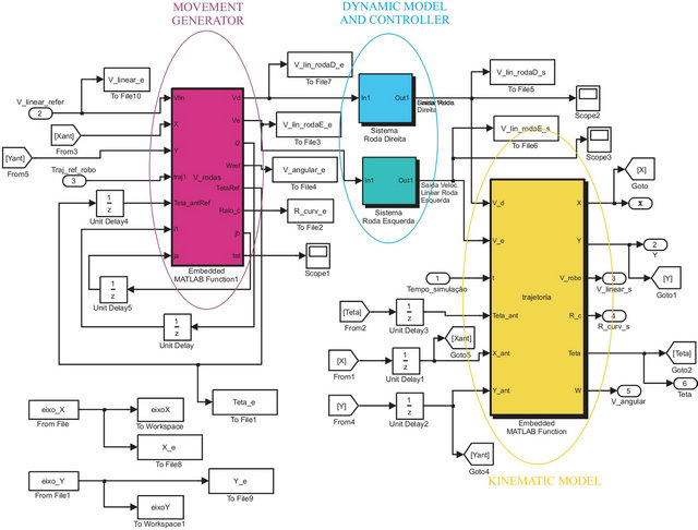
Figure 8. Mobile robot control strategy implemented into Matlab Simulink.
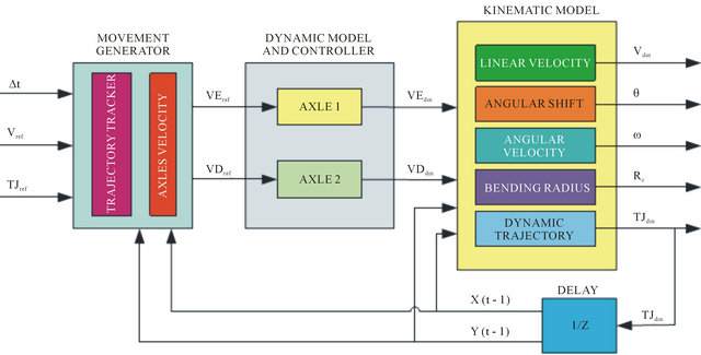
Figure 9. Blocks diagram representing generation modules for movement, controller, kinematic model and dynamic model.
embedded control system, located in the mobile robot, and the beacons, that are located in strategically points in the environment, are composed of a frame formed for five quaternary codes.
5.1. Communication Protocol
The timing diagram shown in the Figure 10 illustrates as each one of the codes in function of clock signal is formed.
Each half clock period correspond to a time about 896 µs. Each code has a time period composed of 8 clocks cycles, that is 14.336 ms. Table 1 AC depicts in a logic way the formation of the codes.
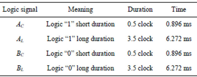
Each code is configured by a logic signals sequence, each one with a determined period. Table 2 shows how each logic signal of each code is composed. The idea is to mount a quaternary codifier using binary logic levels, associates in such way that the logic levels alternate and the total period of each code is the same.
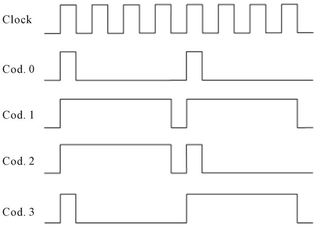
Figure 10. Communication protocol codes.
Table 1. Logic formation of each code.
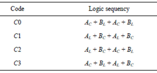
Table 2. The timing of the logic codes.
The codification implemented was conceived here aiming the minimizing of the errors, such as the transmission of the one exactly signal level is transmitted without transitions of level for long time periods. In this case, the receiver tends to put out of the way and to perform the reading out the correct point, originating errors. In this way, RF transmission of the codes is sufficiently robust and trustworthy, practically extinguishing errors of signal decoding signal inside the area of system range.
5.2. The Communication Frame
The communication frames used between the mobile robot and the beacons are composed for five quaternary codes. The Figure 11 illustrates an example of a communication protocol frame. As each code has a period about 14.336 ms, the all frame has transmission time about 71.68 ms.
The maximum number of possible combination is given by

Each beacon has its own address, composed by five codes. In this way, the system is able to deal with up to 1024 beacons, with their own individual address.
5.3. The RF Link
The coded signal is transmitted in RF modulated by BASK-OOK technique. The carrier signal frequency is about 433.92 MHz (UHF band). The RF link uses a halfduplex channel between mobile robot and beacons. The mobile robot control system is previously programmed with quantity and address of each beacon. Figure 12 depicts an example of environment configuration of the communication between the robot and beacons.
5.4. Beacon Transceiver System
The beacon embedded system is composed basically by two modules. One is responsible for RF signal receive and make all the concerned computation. This module has a 16F630 PIC microcontroller, operating at 4 MHz clock frequency. The other one is the RF signal transmitter. This module is equipped with 12F635 microcontroller and also operates at 4 MHz. The system is able to operate in autonomous way, been programmed with specific address. In other hand, the mobile robot must be programmed with de amount and the address of all operative beacons inside the navigating environment. Figure 13 depicts the block diagram of the RF transceiver at mobile robot and at beacons.
| C2 | C0 | C1 | C3 | C0 |
Figure 11. Example of a communication protocol frame.
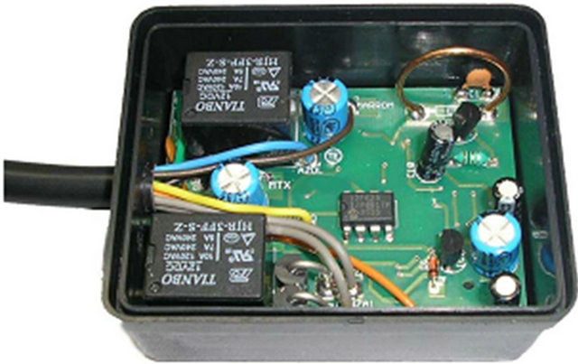
Figure 14 shows the beacons RF transceiver modules. The transmission module (Figure 14(b)) is able to function in asynchronous independent way, emitting an address code frame in a certain period of predetermined time, or synchronous way commanded by the reception and control module (Figure 14(a)). In the first case, a battery 12V A23 model is used which allows autonomy of more than 3 months of continuous use, due to ultra low power energy consumption given by the embedded microcontroller with nanowatt technology. In second case the power supply and transmission command are made by the reception control module, illustrated in the Figure 14(a). This second one is the mode utilized by this work.
As much the mobile robot, as each one of the beacons, has a transceiver control system com-posed by reception module and transmission module. As the objective of our system is to provide a triangulation between the mobile robot position and the beacons, the transmission modules work in synchronous way. It is assumed that the module of control of reception-transmission of the mobile robot has been previously loaded with the amount of existing beacons in the environment and with its respective addresses codes. The functioning of the system goes to the following procedure:
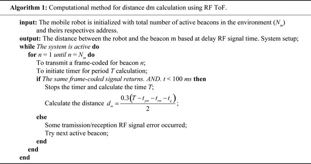
1) The mobile robot emits a address code-frame for first beacon. In this instant it sends an interrupt control signal to the central processing unit for triggering and starts a timer counter. The robot then, waits the return of the signal. This return must occur in up to 100 ms.
2) If the signal returns, means that the beacon recognized the code and sent back the same code. In this instant is sent a signal to the robot embedded central processing unit for stops the timer and calculation of the signal return delay time, which could be about ns.
3) If the signal was not returned, means that the beacon is out of area reach or occurred some error in signal transmission-reception.
4) Increment the number of beacon and go to the loop first item.
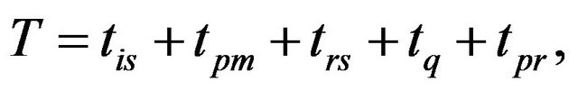
The distance between the robot and a certain m beacon is computed with base of the delay time in the reception of the same transmitted code. The total elapsed time between the code final transmission, sent by the robot, and the reception of the same code, sent back to the beacon, can be calculated by
 (6)
(6)
where tis is the travel signal time between leaves robot transmitter and reach beacon reception, tpm is the processing signal time by the beacon, trs is the signal return elapse time, tq is the frame code period and tpr is the processing time of the sent back signal received by robot.
It’s well known that RF signal cover one meter in about 3.3 ns because its velocity is about 0.3 m/ns in air. We can consider that the linear speed of the robot is so small that the displacement of the robot could be considering as being zero during the time T. In this way, the distance in meters between the mobile robot and the beacon m can be given by
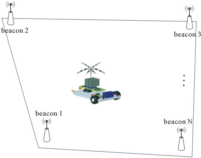
Figure 12. An example of environment beacons arrangement and the communication system.
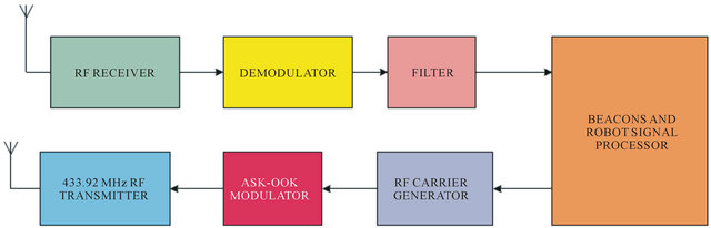
Figure 13. Block diagram of the RF transceiver at mobile robot and at beacons.
 (7)
(7)
where tis and trs are given in ns. The elapsed time T is computed with a 64 bits timer of the Texas Instrument TMS320C6474-1200 dual core robot embedded processor. The instruction cycle time of it is about 0.83 ns (1.2 GHz clock Device), allowing timer calculations in order of ns, essential for our case of study. The times tpm and tpr are determined empirically and tq = 71.68 ms. In this way, the covered distance between the robot and beacon m should be done by
 (8)
(8)
The Algorithm 1 depicts the computation method for distance d calculation using RF ToF.
6. Triangulation
Triangulation refers to the solution of constraint equations relating the pose of an observer to the positions of a set of landmarks. Pose estimation using triangulation methods from known landmarks has been practiced since ancient times and was exploited by the ancient Romans in mapping and road construction during the Roman Empire. The simplest and most familiar case that gives the technique its name is that of using bearings or distance measurements to two (or more) landmarks to solve a planar positioning task, thus solving for the parameters of a triangle given a combination of sides and angles. This type of position estimation method has its roots in antiquity in the context of architecture and cartography and is important today in several domains such as survey science.
Although a triangular geometry is not the only possible configuration for using landmarks or beacons, it is the most natural [2]. Although landmarks, beacons and robots exist in a three-dimensional world, the limited accuracy associated with height information often results in a two-dimensional problem in practice; elevation information is sometimes used to validate the results. Thus, although the triangulation problem for a point robot should be considered as a problem with six unknown parameters (three position variables and three orientation variables), more commonly the task is posed as a twodimensional (or three-dimensional) problem with twodimensional (or three-dimensional) landmarks [8].
Depending on the combinations of sides (S) and angles (A) given, the triangulation problem is described as “side-angle-side” (SAS), and so forth. All cases permit a solution except for the AAA case in which the scale of the triangle is not constrained by the parameters. In practice, a given sensing technology often returns either an
 (a)
(a)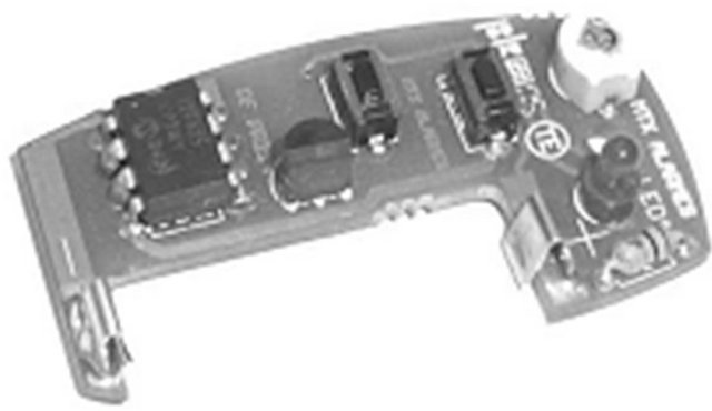 (b)
(b)
Figure 14. Beacons RF transceiver modules. (a) Implemented reception module; (b) Implemented transmission module.
angular measurement or a distance measurement, and the landmark positions are typically known. Thus, the SAA and SSS cases are the most commonly encountered. More generally, the problem can involve some combination of algebraic constraints that relate the measurements to the pose parameters. These are typically nonlinear, and hence a solution may be dependent on an initial position estimate or constraint [9]. This can be formulated as
 (9)
(9)
where the vector x expresses the pose variables to be estimated (normally, for 2D cases ), and
  is the vector of measurements to be used. In the specific case of estimating the position of an oriented robot in the plane, this becomes
 (10)
(10)
If only the distance to a landmark is available, a single measurement constrains the robot’s position to the arc of a circle. Figure 15 illustrates perhaps the simple’s traingulation case.
A robot at an unknown location x1 senses two beacons P1 and P2 by measuring the distances d1 and d2 to them. This corresponds to our case of study in which active beacons at known locations emit a signal and the robot obtains distances based on the time delay to arrive at the robot. The robot must lie at the intersection of the circle of radius d1 with center at P1, and with the circle or radius d2 with center at P2. Without loss of generality we can assume that P1 is at the origin and that P2 is at . Then we have
 (11)
(11)

Figure 15. Simple triangulation example. A robot at an unknown location x1.
and
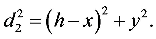 (12)
(12)
A small amount of algebra results in
 (13)
(13)
and
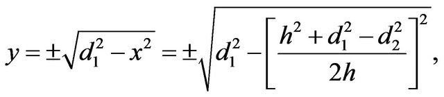 (14)
(14)
resulting in two solutions x1 and x2.
In a typical application, beacons are located on walls, and thus the spurious (in our example, the x2) solution can be identified because it corresponds to the robot’s being located on the wrong side of (inside) the wall. Although distances to beacons provide a simple example of triangulation, most sensors and land-marks result in more complex situations [10]. The situation for two beacons is illustrated in Figure 16(a). The robot senses two known beacons and measures the bearing to each beacon relative to its own straight ahead direction. This obtains the difference is gearing between the directions to the two beacons and constrains the true position of the robot to lie on that portion of the circle shown in Figure 16(a). We can note that the mathematics admits two circular arcs, but one can be excluded based on the left-right ordering of the beacon directions [11]. The loci of points that satisfy the bearing difference is given by
 (15)
(15)
where d1 and d2 are the distances from the robot’s current position x to beacons P1 and P2, respectively. The visibility of a third beacon, like can be seen at Figure 16(b), gives rise to three nonlinear constraints on d1, d2 and d3: by
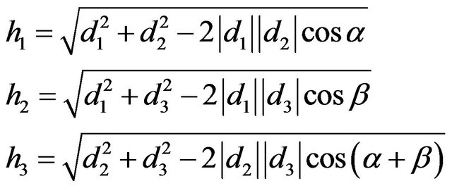 (16)
(16)
which can be solved using standard techniques to obtain d1, d2 and d3. Knowledge of d1, d2 and d3 leads to the robot’s position [1].
The geometric arrangement of beacons with respect to the robot observer is critical to the accuracy of the solution. A particular arrangement of beacons may provide high accuracy when observed from some locations and low accuracy when observed from others. F or example, in two dimensions a set of three collinear beacons observed with a bearing measuring device can provide good positional accuracy for triangulation when viewed from a
 (a)
(a) (b)
(b)
Figure 16. Location estimative of the mobile robot based on beacons triangulation. (a) Triangulation with two beacons; (b) Triangulation with three beacons.
point away from the line joining the beacons (e.g., a point that forms an equilateral triangle with respect to the external beacons). On the other hand, if the robot is located on the line joining the beacons, the position can only be constrained to lie somewhere on this (infinite) line.
6.1. Triangulation with RF Beacons
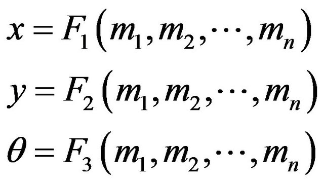
In our case of study the beacon’s position at 2D environment are known and thus, the distances between the beacons. If the N beacons are positioned at points  and the robot’s position is given by
 , then, the Equation (16), that express the robot triangulation with three beacons, yields
 (17)
(17)
where the robot’s position  can be inferred by numerical methods.
6.2. Some Triangulation Results
It’s our choice to make triangulation using a set of tree active environment beacons at a time. In this way, the embedded robot control computes distances d1, d2, d3 from beacons b1, b2, b3 respectively. When those measurements are done, it calculates the robot position estimative, based in Equations (16) and (17). Then, it takes next tree actives beacons, such as b2, b3, b4 with their respective robot distances, for next triangulation. The triangulation keeps in loop reaching last beacon, return to first one and go on.
We noted that, when mobile robot positions was taken in this way, and when the robot get so close form some beacon, at least less then tree meters, the position estimative get corrupt by this near beacon.
That’s because timer counter becomes imprecise for the short distance that results some ns of ToF. Figure 17 depicts a robot trajectory inside a indoor 20 × 21 m environment that triangulation calculus was taken in period of 10 s each one. It does madden in this way, for better robot position estimative visualization.
In the way to fix the robot position estimative when it’s at some beacon nearly, the embedded control simply discards distance measurement from beacons that are less than four meters from robot. That’s why it’s important more than four beacons at indoor environment and best arrangement of them, taking into account obstacles and environment own particularities. Figure 18 illustrates the robot position estimative when this methodology is applied. We can note here that position estimative is now more consistent.
7. Data Fusion
The question of how to combine data of different sources generates a great quantity of research in the academics
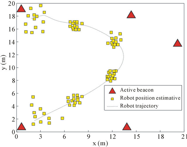
Figure 17. Robot position estimative by beacons triangulartion using all actives beacons.
ambient and at the research laboratories. In the context of the mobile robotic systems, the data fusing must be affected in at least three distinct fields: arranging measurements of different sensors, different positions, and different times.
Here is presented the data fusion methodology that uses Kalman Filter to combine sensors measurements and beacons distance triangulation to have best next pose estimation and correct actual robot localization.
Kalman Filter
To control a mobile robot, frequently it is necessary to combine information of multiple sources. The information that comes from trustworthy sources must have greater importance about those one collected by less trustworthy sensors.
A general way to compute the sources that are more or less trustworthy and which weights must be given to the data of each source, making a weighed pounder addition of the measurements, are known with Kalman Filter [12]. It is one of the methods more widely used for sensorial fusing in mobile robotics applications [13]. This filter is frequently used to combine data gotten from different sensors in a statistical optimal estimate. If a system can be described with a linear model and the uncertainties of the sensors and the system can be modeled as white Gaussian noises, then the Kalman Filter gives an optimal estimate statistical for the casting data. This means that, under certain conditions, the Kalman Filter is able to find the best estimative based on correction of each individual measure [14]. Figure 19 depicts the particular schematic for Kalman Filter localization [15].
The Kalman Filter consists of the stages follow presented in each time step, except for the initial step. It is assumed, for model simplification, that the state transition matrix  and the observation function
  remain constant in function of the time. Using the plant model and computing a system state estimate in the time
  based in robot position knowledge in the instant of time k, is had how the system evolves in the time with the input control
 :
:
 (18)
(18)

Figure 18. Robot position estimative by triangulation with best beacons position.
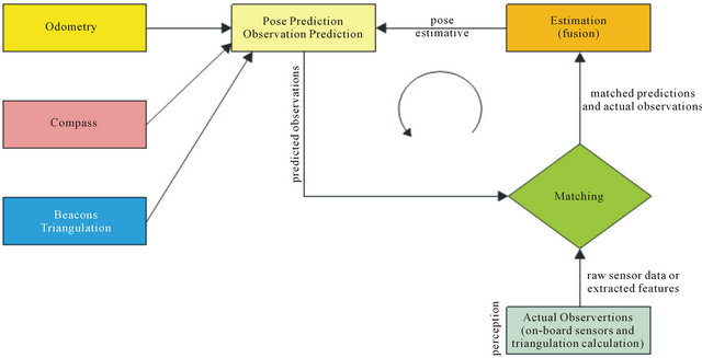
Figure 19. Schematic for Kalman Filter mobile robot localization.
In some practical equations the input  is not used. It can also, to actualize the state certainty as expressed for the state covariance matrix
  through the displacement in the time, as:
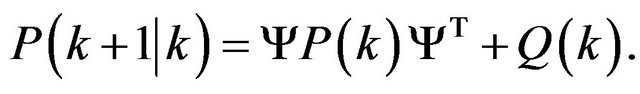 (19)
(19)
Equation (19) expresses the way which the system state knowledge gradually decays with passing of the time, in the absence of external corrections. The Kalman gain can be express as
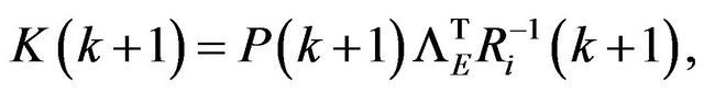 (20)
(20)
but, how it didn’t compute , this can be computed by
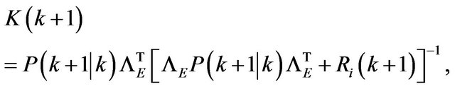 (21)
(21)
Using this matrix, an estimate of revised state can be calculated that includes the additional information gotten by the measurement. This involves the comparison of the current sensors data  with the data of the foreseen sensors using it state estimate. The difference between the two terms:
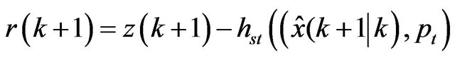 (22)
(22)
or, at the linear case
 (23)
(23)
is related as the innovation. If the state estimate is perfect, the innovation must be not zero only which the sensor noise. Then, the state estimate actualized is given by
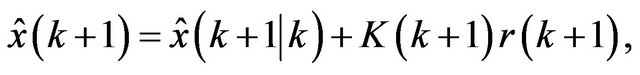 (22)
(22)
and, the up-to-date state covariance matrix is given by
 (23)
(23)
where I is the identity matrix.
8. Experimental Results
Here is presented some experimental results of the proposed system. A mobile robot prototype showed in Figure 20 was used as a platform for implementation the hardware and the software above described.
We can see at Figure 21 the result of EKF pose estimative applied in the robot’s trajectory that have traingulation measurements marked by yellow crosses. In this experimental result we allocate four beacons, one in each corner, about two meters high. In the middle of the room, there was a camera for registering the true robot’s trajectory in the way to comparison.
The ellipses delimit the area of uncertainty in the esti-
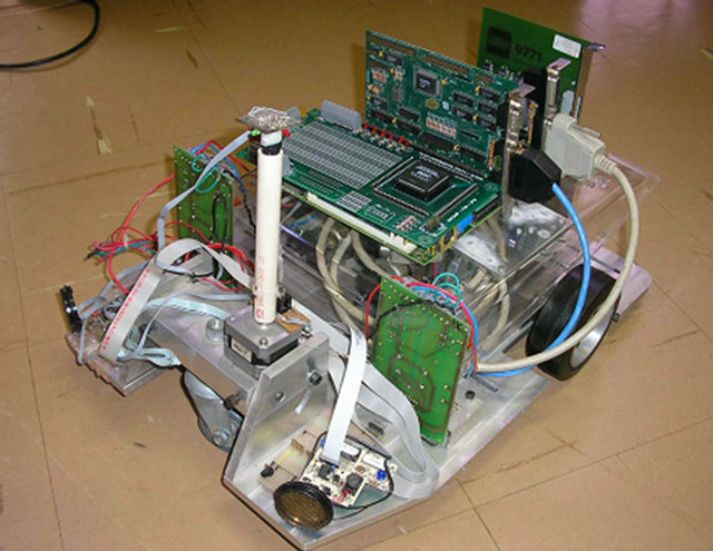
Figure 20. Experimental mobile robot prototype.

Figure 21. The result of EKF pose estimative applied at irregular curvilinear trajectory.
mates. It can be observed that these ellipses are bigger in the trajectory curves extremities, because in these points the calculus of position by triangulation get some loses.
The average quadratic error varies depending on the chosen trajectory. It can be noticed that the pose estimative improves for more linear trajectories and with high frequency of on-board RF beacons triangulation measurements.
Figure 22 depicts the robot navigation inside environment with two ambient. Here were fixed six actives beacons for massive triangulation computation. The trouble with massive triangulation is that the onboard embedded processor keeps busy computing it and has not enough time for others important tasks like wheel control management, supervisory communication, EKF calculation, etc. In this way, it’s important to find a middle term about triangulation measurement frequency that will not
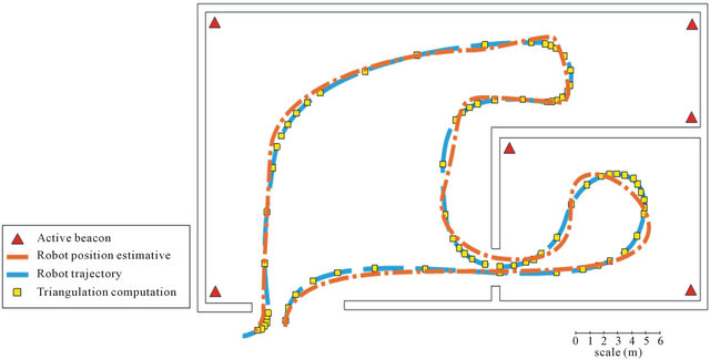
Figure 22. Robot navigation in multiple rooms environment.
compromise the well function of all control embedded system.
9. Conclusions
The use of ToF of the RF signal interacting with RF beacons for computational triangulation in the way to provide a pose estimative at bi-dimensional indoor environment was validated, with those first experimentation works. Even though we are collecting the first positive results in this way, they are encouraging us to keep researching and improving the system in this direction. This is a relativity cheap implementation system that provides grates results for mobile robot indoor navigation, where GPS system is out of range. In this way, this work brings an important alternative for traditional ultrasonic navigation technology, with low cost implementation RF digital transceiver beacon system. These are now possible because of high performance robot embedded multicore DSP processors to calculate ToF of the order about ns.
Sensors data like odometry, compass and the result of triangulation Cartesian estimative, was fused in a Kalman filter in the way to perform optimal estimation and correct robot pose. Once given the nonlinearity of the system in question, the use of the EKF became necessary. It does not have therefore, at beginning, theoretical guarantees of optimality nor of convergence of this method. Therefore, it was implemented a kinematic and dynamic model at embedded control system that allows, underneath of next conditions of the reality, to verify the performance of this technique. Among others parameters that were looked to realistic model the increasing error in the measure of the position of a beacon to the measure meets that in the distance between the robot and it increases. This effect also was introduced in the estimate of the observation covariance matrix to allow a more coherent performance of the filter. A factor extremely important is the characterization of the covariance’s matrices of the present’s signals in the system.
The results of the simulations associated with experimental validations confirm that this technique is valid and promising so that the mobile robots, in autonomous way, can be able to correct its own trajectory. The consistency of the data fusing relative to the odometry and compass sensing of the mobile robot and the result of RF beacons triangulation is obtained even after inserted disturbances in the system. The presented method does not make an instantaneous absolute localization, but successive measurements show that the estimative state converges for the real state of the robot.
REFERENCES
- M. Thielscher, “Reasoning Robots, the Art and Science of Programming Robotic Agents,” Springer, Netherlands, 2005.
- G. Dudek and M. Jenkin, “Computational Principles of Mobile Robotics,” Press Syndicate of the University of Cambridge, Cambridge, 2000.
- S. H. Park and S. Hashimoto, “Autonomous Mobile Robot Navigation Using Passive Rfid in Indoor Environment,” IEEE Transactions on Industrial Electronics, Vol. 56, No. 7, 2009, pp. 2366-2373. doi:10.1109/TIE.2009.2013690
- C.-F. Juang and Y.-C. Chang, “Evolutionary-GroupBased Particle-Swarm-Optimized Fuzzy Controller with Application to Mobile-Robot Navigation in Unknown Environments,” IEEE Transactions on Fuzzy Systems, Vol. 19, No. 2, 2011, pp. 379-392. doi:10.1109/TFUZZ.2011.2104364
- H.-S. Shim, J.-H. Kim and K. Koh, “Variable Structure Control of Nonholonomic Wheeled Mobile Robot,” IEEE International Conference on Robotics and Automation, Vol. 2, 1995, pp. 1694-1699.
- Y. L. Zhao and S. L. BeMent, “Kinematics, Dynamics and Control of Wheeled Mobile Robots,” IEEE International Conference on Robotics and Automation, Vol. 1, May 1992, pp. 91-96.
- N. MacMillan, R. Allen, D. Marinakis and S. Whitesides, “Range-Based Navigation System for a Mobile Robot,” Conference on Computer and Robot Vision (CRV), 2011, pp. 16-23.
- H. Gonzalez-Banos and J.-C. Latombe, “Robot Navigation for Automatic Model Construction Using Safe Regions,” Experimental Robotics VII, Lecture Notes in Control and Information Sciences, Vol. 271, 2001, pp. 405- 416. doi:10.1007/3-540-45118-8_41
- M. Kam, X. X. Zhu and P. Kalata, “Sensor Fusion for Mobile Robot Navigation,” Proceedings of the IEEE, Vol. 85, No. 1, 1997, pp. 108-119. doi:10.1109/JPROC.1997.554212
- A. N. Tikhonov and V. Y. Arsenin, “Solutions of Ill-Posed Problems,” Wiston, Washington DC, 1977.
- M. Thielscher, “Reasoning Robots. The Art and Science of Programming Robotic Agents,” Springer, Netherlands, 2005.
- R. E. Kalman, “A New Approach to Linear Filtering and Prediction Problems,” Journal of Basic Engineering, Vol. 82, No. 1, 1960, pp. 35-45. doi:10.1115/1.3662552
- J. J. Leonard and H. F. Durrant-Whyte, “Mobile Robot Localization by Tracking Geometric Beacons,” IEEE Transactions on Robotics and Automation, Vol. 7, No. 3, 1991, pp. 376-382. doi:10.1109/70.88147
- G. Dudek, M. Jenkin, E. Milios and D. Wilkes, “Reflections on Modelling a Sonar Range Sensor,” 1996.
- R. Siegwart and I. R. Nourbakhsh, “Introduction to Autonomous Mobile Robots. Intelligent Robotics and Autonomous Agents,” The MIT Press, 2004.