Journal of Geographic Information System
Vol.6 No.4(2014), Article
ID:48527,10
pages
DOI:10.4236/jgis.2014.64028
Overcoming Object Misalignment in Geo-Spatial Datasets
Ismail Wadembere*, Patrick Ogao
College of Computing and Information Science, Makerere University, Kampala, Uganda
Email: *wadembere@gmail.com
Copyright © 2014 by authors and Scientific Research Publishing Inc.
This work is licensed under the Creative Commons Attribution International License (CC BY).
http://creativecommons.org/licenses/by/4.0/


Received 9 June 2014; revised 5 July 2014; accepted 29 July 2014
ABSTRACT
In integrating geo-spatial datasets, sometimes layers are unable to perfectly overlay each other. In most cases, the cause of misalignment is the cartographic variation of objects forming features in the datasets. Either this could be due to actual changes on ground, collection, or storage approaches used leading to overlapping or openings between features. In this paper, we present an alignment method that uses adjustment algorithms to update the geometry of features within a dataset or complementary adjacent datasets so that they can align to achieve perfect integration. The method identifies every unique spatial instance in datasets and their spatial points that define all their geometry; the differences are compared and used to compute the alignment parameters. This provides a uniform geo-spatial features’ alignment taking into consideration changes in the different datasets being integrated without affecting the topology and attributes.
Keywords:Object-Based, Geometry Alignment, Geo-Spatial Management

1. Introduction
The appreciation of geo-spatial information by the different information system managers and users as the basis for location based decision-making has led to the need to develop approaches for integrating geo-spatial datasets as the driving force towards the vision of common data storage to increase availability and accessibility of already captured geographic information through exchange and sharing. Most geo-spatial information systems use map layers to organize geographical and geo-spatial objects forming features in datasets. Each layer describes a certain aspect of the modeled real world e.g. roads, buildings, forest, etc. This provides a natural technique to organize and visualize data from different sources making it an efficient way of data storage, manipulation, and analysis [1] .
Features especially on earth’s surface and land uses are constantly changing, so is the need to continuously update, adjust, and align the objects forming features on different layers in geodatabases. These layers are always updated separately by individuals or organizations concerned with certain aspects and locations. However, storing map layers separately makes it difficult to directly solve topological queries that relate to features that belong to many and different layers [1] and [2] , thus the need to integrate using algorithms based on either geometric matching, topological matching, or semantic matching [3] . However, because of the various and multisources of data, method of collection, instrument used, method of storage, and projection parameters used, the different geo-spatial datasets sometimes cannot match perfectly. In the process, overlay operations intersect objects from different layers resulting into creation of new objects that are unwanted [2] or leave opening between features. This does not accomplish the need of integrating datasets since it leaves the geodatabases not properly updated with the required new changes to depict what is currently on the ground.
To overcome that, object-based geometry adjustment algorithms [2] -[6] have been developed that can be used to adjust features. In this paper, we use these algorithms combining them in different ways to come up with individual object-based geo-spatial data alignment method so that complementary and adjacent datasets can be integrated without creating overlaps, openings, undershoots, and overshoots that result into slivers (unwanted small objects) and danglings (duplicate points, lines, or polygons) in geo-spatial datasets.
2. Related Work
2.1. Dataset Integration
Geo-spatial datasets are captured using different methods, instruments, reference systems and geodetic datum that make datasets to vary. Thus, different operations and many algorithms exist for carrying out clipping and finding intersection between two datasets. Some focus on merging similar geometric objects [3] including exchange of attributes or for homogenizing geometry. This address semantics heterogeneity of spatial datasets, improvement of quality in case one dataset is captured to a higher quality, multi representation based on the matching of two datasets using Unified Modeling language (UML), selecting matching objects using Structured Query Language (SQL), and geo-spatial object geometry adjustment. For polygon overlays, many algorithms are explained by [2] and [4] that can work on different polygons like convex, rectangle, and concave polygons with some requiring complex and specific data structures and others computing Boolean operations on polygons that help to determine the intersection of segments [2] . Although these operations determine the spatial coincidence (if any) of two data layers, they do not guide the end user on how to implement them to update geo-spatial datasets through aligning features for same, adjacent, or complementary datasets.
For the approaches that handle combined primitives, we find a huge number of research efforts in this domain: 1) approaches dealing with geo-spatial object matching, and 2) methods for geo-spatial object intersection or database updating. Different schemes have been proposed: a) layer’s overlying approaches that use algorithms for different geo-spatial data merging tasks, and b) more specific ideas, using individual geo-spatial object adjustment strategies, to achieve full integrated solution. The latter is the focus of this work dealing with geometry alignment basing on current approaches like Boolean polygon matching [2] , alignment algorithms [5] , computational geometry [7] , and object adjustment in corresponding datasets [6] .
2.2. GIS Vector Data Structure and Composition
There are two common spatial data models for geo-spatial data storage—raster and vector. In the alignment method, we focus on vector, which is the use of directional lines to represent a geographic feature. Several different vector data models exist, however only two are commonly used in GIS data storage: computer-aided drafting (CAD) and topologic data structure. The focus is on topologic since it maintains spatial relationships among features. Three files types are considered: 1) shapefile as it has been around since the 1980s and remains one of the most common data transfer formats, 2) GML is text and is human readable, and 3) Spatialite as it uses one file and is able to store geometries and query them with spatial functions similar to what is found in geodatabase like PostGIS.
As we developed method, we link topological data structures to the requirement of geo-spatial framework:
1) The ideal method for improving data usability should be based on object-oriented data model [8] [9] . The geo-spatial data must be modeled as identifiable objects according to the geographic entities (features) existing in the real world, which helps to link spatial information with various social-economic and natural resource information.
2) Geo-spatial data from different sources with varying scales must be able to be mapped to the same standards, data model, projection, and representation [10] [11] so that the description of the same entity in different datasets is consistent.
3) The relationships among objects should be modeled and integration of different geo-spatial datasets must handle the three dimension 1) horizontal (adjacency), 2) vertical (overlay), and 3) temporal (time) integration [12] , for example, the relations among buildings and land plots, the relations between poles (point object) and electricity line (line object) [13] , etc.
The alignment method uses the three characteristics where objects forming features are used as the modeling unit basing on the primary spatial primitives (point, polylines, and polygons) to accomplish the geometrical inconsistency correction through updating and adjustment of objects so that they align in the three dimensions (horizontal, vertical, and temporal) of spatial data. This is done by putting into consideration the desirable characteristics of information systems—being true, up-to-date, standard, flexible, concise, in desired form and sufficient to the needs of users and their need to share [14] . For GIS, sharing provides avenues to distribute geographic information among many users which enhances decision-making and produces significant savings in data collection and merging by reducing the effort and money wasted as result of duplication [15] [16] , which is the aim of many initiatives like openstreepmap, googlemaps, OpenGIS, and SDI. The alignment method compliments these initiatives by making it easy to update, adjust, and align geometries of objects in dataset horizontally, vertically and over time in line with the second and third characteristics of geo-spatial framework.
3. The Alignment Method Requirements
Geo-spatial data alignment approaches are categorized into global and local/individual. Global methods assume that all features on layer can be aligned using the same parameters. Methods like “automatic image-map alignment problem using a similarity measure named edge-based code mutual information” [5] are good for image based datasets and use global transformation parameters that do not take care of individual object changes. Others include vector based polygon clipping, intersection, or overlay [2] and [4] . The individual methods assume that each feature on layer may have different errors and alignment parameters are computed for each object like alignment method.
For vector GIS data alignment, there are certain requirements that have to be fulfilled
• maintain the meaning of the shapes—this calls for keeping the attributes;
• maintain the relationship between objects—this is handled under topology;
• separate data into layers for easy modeling and analysis—need to keep objects on layers during alignment.
We added the following to guide in development of alignment method.
• it should be possible to handle individual objects on a layer or parts of objects;
• able to handle points, lines, and polygons or any combination of them.
There are requirements and conditions that must be fulfilled and should exist in datasets during and after alignment method, these are categorized into four: datasets merging requirement, geo-spatial complementary alignment, datasets transformation requirement, and aligned datasets characteristics.
During integration, there are certain dataset merging requirements that need to be satisfied to have a proper GIS vector dataset or layer.
• There should be no slivers (small-unwanted objects) that result from objects intersecting during merging of datasets. If slivers do appear, they should be adjusted during alignment instead of using clean or removal algorithms to eliminate them;
• There should be no danglings (meaningless points and lines) in the final aligned dataset. Nodes should only exist at the end of lines or at intersection of lines. Vertices should only be along a line where there is change of direction;
• Merging should take place on datasets in the same projection, scale, and datum;
• Merging is should be based on objects forming features and primary attribute used for identification.
We introduced the term “geo-spatial complementary alignment” to define three different situations that can exit during geometry adjustment and alignment between Adjustment Dataset (AD) and Reference Dataset (RD). Where AD is dataset that need updating or has objects that need to be adjusted while RD is the dataset used as reference during computing of adjustment and alignment parameters:
1) Single Forward Alignment (SFA): where RD has all the details required to update AD and only comparison with AD is needed to compute alignment parameters. Let us take an example of two datasets—AD having residential plots and RD with both residential plots and houses on those plots. If RD has all recent information on houses needed for AD, then the updates for SFA will be applied where values from RD are transferred to AD and nothing is brought backwards to RD.
2) Single Complementary Alignment (SCA): RD does not have all the required details to update and adjust objects in AD. This means there is need to get some details from AD to supplement on those coming from RD before final alignment of AD can be achieved even when the dataset of interest is AD. For example RD has recent information on houses and AD has proper demarcation of land plots for the houses. The two are needed in order to get updated dataset having plots with properly aligned and corresponding houses.
3) Two-way Complementary Alignment (TCA): Neither RD nor AD have all the required details to stand alone, but both need to be updated. This means that there is need to get details from the two to update each for both to be useful. For example AD has recent information on houses and RD has proper demarcation of land plots for the houses, but we need both datasets to be updated. Another example is where RD and AD are adjacent, but the two need to be updated to obtain a perfect boundary without creating openings and overlaps.
There are dataset transformation requirements that the resulting datasets should satisfy including:
• Objects and features can maintain their meaning (primary attributes);
• Transformation can change the meaning of object if it is needed;
• Transfer of primary attribute can be between two different datasets;
• The relationship between objects should be kept;
• Transformation can move datasets from one projection to another;
• Transformation can change geometry primitive type if needed;
• Coordinates of objects can be changed during transformation;
• Coordinate systems can be changed during transformation;
• Transformations can move datasets from one datum to another;
• Transformations can change the number of objects in layer or dataset through addition or deletion.
The characteristics of aligned datasets include the following:
• shapes having meaning (primary attribute);
• relationship between object maintained;
• data able to be separated into layers for easy modeling and analysis;
• able to identify individual objects or parts of object on a layer;
• no slivers and danglings;
• final projection being that of the reference dataset.
4. The Components of the Alignment Method
The object-based geometry adjustment algorithms [2] -[6] were used in varying combinations according to the requirements as detailed in previous Section 3. They were manipulated to get the four major components of the alignment method 1) data input, 2) data preparation (cleaning, matching, geometry validity, and primary attribute), 3) data processing, and 4) data management as shown on Figure 1—the method flowchart.
4.1. Data Input
The first task is reading the geo-spatial datasets involved in the alignment as layers—reference dataset (RD) that will provide alignment values and adjustment dataset (AD) that has objects to be aligned. The user specifies the AD and RD, also identifies the primary attribute (PA) which is the meaning of features. As the data is read in, the data structures are compared to check for geometry type of objects (points, lines, polygons) before storing them in matrices according to their geometry type. This is vital to ensure that same geometry type are used when comparing, updating, adjusting, and aligning datasets.
4.2. Data Preparation
Data preparation involves putting the data into the same projection, cleaning and removing unnecessary geome-
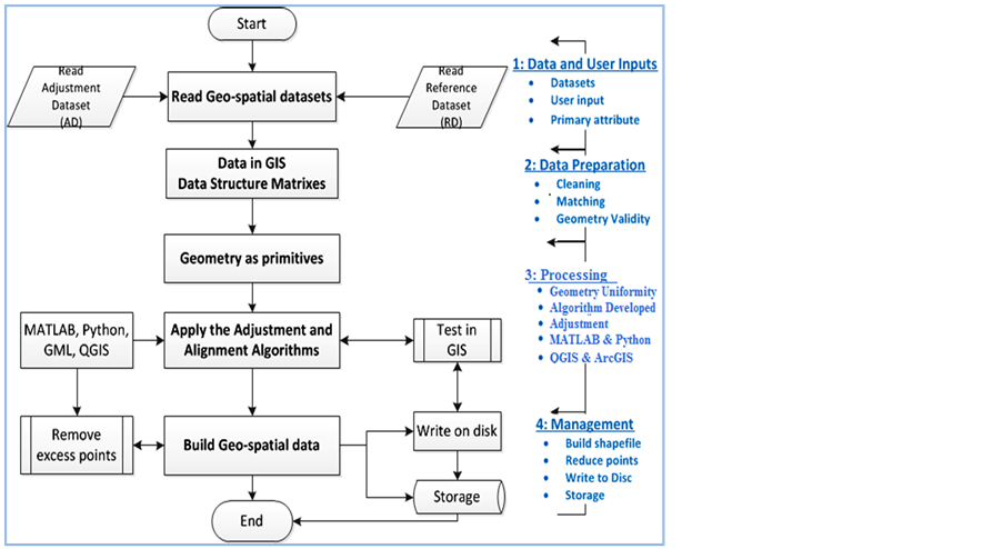
Figure 1. Alignment method components and flowchart.
tries, matching the corresponding object in the datasets, difference determination, and making sure that geometries being worked on are the same—point with point, line with line, and polygon with polygon. This is achieved by algorithms based either on geometric, topological, or semantic matching [3] . For the GIS data layers the difference is determined and parameters used in comparison are precision, resolution, and actual data values. Those steps are already available in the existing GIS applications like QGIS, ArcGIS, and Jump GIS.
If the difference obtained is zero, that means the layers are the same and objects do match. If the result is not zero, it could be positive or negative, that means the two datasets have variations. The positive or negative values indicate the direction, to either subtract or add during the geometrical adjustment. It helps also in identifying the objects that are causing the differences. For positive, it means the first dataset have bigger or more geometry components and vice versa for negative. Implying that for the positive, either geometry objects have to be reduced in the first dataset or more objects have to be added in the second dataset. For negative it means they are more or bigger objects in the second dataset thus the need to add in the adjustment dataset if requirement is only to update or to reduce in the second (reference dataset) in case of complementary.
To apply the above, the method takes advantage of the way geo-spatial datasets are organized according to meaning (themes). Each theme is stored independently in layers like road layer having types of roads (like highways, avenues), building layer having different buildings (like houses, plazas, gatehouse, arcades, etc.). This provides a natural way and technique to organize and visualize data from different sources making it an efficient way of data storage, manipulation, and analysis [1] . For gatehouse on a building layer, there are objects like window, door, etc. that are represented by spatial objects. The objects are defined by their shape, size, and location presented by primitives (points, lines, and polygons). The vertices define the shape of the polyline along its length. Polylines that connect to each other will share a common node. Polygons are formed by bounding polylines that keep track of the location of each polygon.
4.3. The Processing
During the processing, the requirements vary from one dataset to another. That is why each algorithm is able to run and be called upon to act independently depending on the complementary situations and adjacent requirements.
The method translates and decodes the geometry shape into text by reading and creating the data structure followed by storing the text in a matrix. In MATLAB, the function “shaperead” handles the reading of layers and it populates matrixes, for example S = shaperead (“nakawa.shp”)—reads the nakawa layer and keeps the matrix in variable S. The alignment method creates a data structure if needed for example using “struct” function in MATLAB S = struct (“Geometry”, “Line”, “Bounding Box”, [0 0; 3 3], “X”, [1 2 2 1 1], “Y”, [1 1 2 2 1]). To reference and work on a particular spatial point in a matrix, the approach of specifying its row and column number is used, where in the matrix variable S, specify the row then column: S (row, column). The number of objects inside the structure is computed and is used to determine the number of iterations to perform on the structure during the alignment process. Since the x-y coordinates for points, vertices, and nodes of all objects forming features on a layer are read, geometry adjustment takes place by changing the x-y values that are handled in their respective indexes as variables to ensure the objects and shape can be reconstructed.
The method takes advantage of the geometries editing in a text form and the following capabilities are provided:
1) Creation of points, lines, and polygons;
2) Moving points, lines, and polygons;
3) Deleting points, lines, and polygons;
4) Inserting, moving, and deleting vertices;
5) Combining and exploding of geometries to and from datasets.
The alignment method runs in such a way that it loads the various adjustment algorithms in different combinations to provide the needed geometry alignment. Different functions in existing algorithms were extracted and grouped into the following sub-algorithms that form the alignment method:
1) Reading the datasets and identifying geometry type;
2) Carrying out dataset to dataset referencing and deciding on type of adjustment;
3) Making the number of objects the same in the two datasets;
4) Updating, adjusting, and aligning the geometries using coordinate values;
5) Writing the aligned dataset onto disk.
To put the method into action, we used Nakawa shapefiles having many but varying objects. The data sources were KCCA (Kampala City Council Authority) and UBOS (Uganda Bureau of Statistics) representing Nakawa division of Kampala City in Uganda as shown on Figure 2.
From the above figure, we are able to see the size and shape of objects but not their structure details (geometry type, location, number of objects, and attributes). KCCA dataset is used as RD (on left) has smaller sub-divisions called parishes and the one from UBOS used as AD (right) represents Nakawa as one solid object. Using MATLAB (or any data structure details viewer), we extracted the data structure (see Table 1 and Table 2) in order to have the parameters that are updated and adjusted.
In the tables above, we have the file name characters (Filename), types of geometry objects inside (ShapeType), the location extend of the dataset (Bounding Box), number of objects inside (NumFeatures), the number of attributes associated with each structure (Attributes). The dataset from KCCA (Table 1) had 23 objects that can observed by looking at the NumFeatures row and comparing it with Table 2 of UBOS that has only one object. In addition, the dataset from KCCA has more details that can be observed by looking at the attributes as it has 18 columns of attributes as compared to eight columns in the dataset from UBOS. It can also be observed that the two datasets although representing the same location (Nakawa division of Kampala City) lie in different locations according to the min and max values as per Bounding Box of each dataset (Table 1 and Table 2). Extracting the bounding box values and comparing them using Table 3, we observe variation in location.
From table, the two datasets are located between same latitudes as per their Easting (x-coordinates) readings, but in different longitudes (locations) along the northing (y-coordinates) readings. Putting that on the x-y axes, we get Figure 3 that shows relative location of the two bounding boxes for the two datasets.
Further analysis shows that two datasets occupy the same size of area of 9057 by 13755 meters on earth’s surface, although they are at different locations because of varying y-values, they have same x-values. This is common for datasets that have been capture and stored using different systems. That means for the two datasets to lie in the same location and to have the same size of boundary box for the two datasets, method carried out dataset to dataset referencing, that we termed “Dataset Referencing”. This is achieved by translating AD through 9,800,000 meters (difference between the y-values as computed in Table 3) along the y-axis to be at the same location as RD on the earth’s surface. This makes the AD to have the size of the bounding box and to be in the same location as RD.
The next step was to deal with the number objects in the datasets, from Table 1 and Table 2, dataset AD from UBOS had one object, therefore, the number of objects in AD had to be increased to match those of RD. The method accomplishes that by inserting more objects into AD using the coordinates details of the objects in RD.
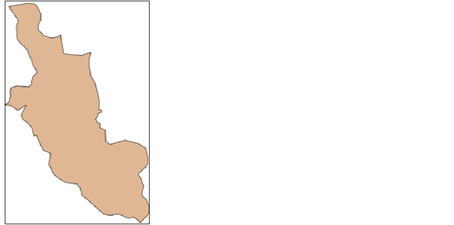

Figure 2. Nakawa from KCCA (left) and UBOS (right).

Figure 3. Location of bounding boxes for Nakawa.

Table 1. Data structure details of Nakawa data from KCCA.
Table 2. Data structure details of Nakawa data from UBOS.
Table 3. Nakawa geometry bounding box.
This is done by handling one object in RD at a time and the process involves reading object’s details that are attached to points (in this case the vertices along the segments that make up the edges of polygons and transferring them into AD. This is done by inserting the x-y values and corresponding attributes into matrix having the AD data structure. The process continues until all objects in RD and their attributes are read and transferred. This makes AD to have the same numbers of objects as RD and its attribute matrix will increase as per number of copied objects. This alignment process accomplishes the updating and adjustment of AD.
Aligning the Updated Objects
The final x-y values obtained after updating and adjustment actions are used to replace the x-y coordinates of objects and fed back into the matrix of the data structure. It should be noted that, it is only x-y values of all the components of data structure that are replaced in the matrix. This helps to maintain the attribute and topology/relationship between the objects in the dataset.
The process continues for each vertex and for each object in the dataset being aligned to get a list of values as:
List of x values (Xuv1, Xuv2, Xuv3, Xuv4… Xuvn)
List of y values (Yuv1, Yuv2, Yuv3, Yuv4… Yuvn)
After changing the x-y values, the method compares the attributes/meaning by promoting the user to identify the primary attribute for each object. If the user decides to add more attributes, then she/he indicates so. The method proceeds by reading the attributes from the matrix and appends them to the attributes in the data structure of the target dataset.
4.4. Management
4.4.1. Converting Updated Objects into a GIS Layer
The aligned objects are transformed from the matrix format into the vector layer and written to the disk. For the case of shapefiles, three files for each shapefile are created with the same base name but varying file extensions. The extensions are .dbf (attribute format—columnar attributes for each shape, in dBase IV format), .shp (shape format—stores the geometry of the objects), and .shx (shape index format—a positional index of the object geometry to allow seeking forwards and backwards quickly). For example a shapefile of districts will have districts.dbf, districts.shp, and districts.shx files.
4.4.2. Point Removal and Bend Simplification
After alignment process, point removal algorithm or bend simplification algorithm maybe applied in case there is need to reduce on the number of points or storage or achieve line generalization [17] . However, care should be put into consideration when using point remove algorithm so the objects do not loss their original geometry shape that in turn affects the topological relations between objects.
4.4.3. Testing the Alignment Method
Testing was carried out using different datasets and conditions as described under requirement of the alignment method, where by adjustment Dataset (AD) was updated and objects adjusted so that they align using correspond-ing reference dataset (RD) values that fed into the method as demonstrated in Section 4.3 using Nakawa dataset.
5. Conclusion and Future Work
5.1. Conclusion
We have shown that geo-spatial data integration can be effectively carried out by incorporating geometry alignment to update and adjust one dataset with changes from another dataset or a known source. This can be easily done by using spatial geometry objects that are manipulated to define all geo-spatial data elements. With this, we obtain a uniform alignment that avoids slivers and danglings that are always created during data merging due to overlaps, openings, and overshoots among geometries of features on layers as a result of variations in data capture, storage, and manipulation approaches. This supplements effective integration of data from a variety of sources that contributes to increased understanding and informed decision-making about actions taking place on earth through answering complex questions in geo-spatial information systems. The method was tested on actual geo-spatial datasets and an analysis of resultant datasets met requirements of topological vector GIS datasets.
5.2. Future Work
To facilitate day-to-day use by GIS practitioners, we plan to convert the method into an application or extension using python that can be used as a plugin in QGIS. This will put all the functionalities into a QGIS menu like “Geometry Alignment” and different functions accessed by QGIS users by clicking on its submenus. The functionalities will come from the different independent algorithms that make up the method. QGIS plugin will have the help that links and explains all functionalities and a well-documented user guide detailing on how to implement all tasks on actual data.
References
- Oosterom, P.V. (1994) An R-Tree Based Map-Overlay Algorithm. EGIS Foundation.
- Martinez, F., Rueda, A.J. and Feito, F.R. (2009) A New Algorithm for Computing Boolean Operations on Polygons. Computers & Geosciences, 35, 1177-1185. http://dx.doi.org/10.1016/j.cageo.2008.08.009
- Moosavi, A. and Alesheikh, A.A. (2008) Developing of Vector Matching Algorithm Considering Topologic Relations. In: Proceedings of Map Middle East, UAE, Dubai, Paper No. 40. http://gisdevelopment.net/proceedings/mapmiddleeast/2008/index.htm
- Liu, Y.K., Wanga, X.Q., Bao, S.Z., Gombosi, M. and Zalik, B. (2007) An Algorithm for Polygon Clipping, and for Determining Polygon Intersections and Unions. Computers & Geosciences, 33, 589-598. http://dx.doi.org/10.1016/j.cageo.2007.03.002
- Li, T. and Kamata, S. (2008) Automatic Image-Map Alignment Using Edge-Based Code Mutual Information and 3-D Hilbert Scan. The Journal of IIEEJ, 37, 223-230.
- Sester, M., G?sseln, G.V. and Kieler, B. (2007) Identification and Adjustment of Corresponding Objects in Datasets of Different Origin. 10th AGILE International Conference on Geographic Information Science 2007, Aalborg University, 1-7.�
- Bayer, T. (2008) The Importance of Computational Geometry for Digital Cartography. Geoinformatics, Faculty of Civil Engineering (FCE), Czech Technical University, Prague. http://geoinformatics.fsv.cvut.cz/gwiki/The_importance_of_computational_geometry_for_digital_ cartography
- Najar, C., Rajabifard, A., Williamson, I. and Giger, C. (2006) A Framework for Comparing Spatial Data Infrastructures An Australian—Swiss Case Study. GSDI-9 Conference Proceedings, Santiago, 201-213.
- Usery, E.L. (1996) A Conceptual Framework and Fuzzy Set Implementation for Geographic Features. In: Burrough, P. and Frank, A., Eds., Geographic Objects with Indeterminate Boundaries, GISDATA Series Vol. 2, Taylor and Francis, London, 71-86.
- Friis-Christensen, A., Nytun, J.P., Jensen, C.S. and Skogan, D. (2005) A Conceptual Schema Language for the Management of Multiple Representations of Geographic Entities. Transactions in GIS, 9, 345-380. http://dx.doi.org/10.1111/j.1467-9671.2005.00222.x
- Parent, C., Spaccapietra, S. and Zimanyi, E. (2005) Modeling and Querying Multi-Representation Spatio-Temporal Databases Information Systems. Information Systems, 31, 733-769.
- Chrisman, N.R. (1990) Deficiencies of Sheets and Tiles: Building Sheetless Databases. International Journal of Geographical Information Systems, 4, 157-167. http://dx.doi.org/10.1080/02693799008941537
- Jiang, J., Chen, J., et al. (2005) A Model for Integrating Multi-Scale Spatial Data for e-Government and Public Service. SDI and Web Services. From Pharaohs to Geoinformatics, FIG Working Week 2005 and GSDI-8, Cairo.
- Erdi, A. and Sava, D.S. (2005) Institutional Policies on Geographical Information System (GIS) Studies in Turkey. Pharaohs to Geoinformatics, FIG Working Week 2005 and GSDI-8, Cairo.
- Sohir, M.H. (2005) The Role of ESA in Building the Egyptian Spatial Data Infrastructure (ESDI) towards the Electronic Government (E-gov.). Spatial Portals and e-Government. From Pharaohs to Geoinformatics, FIG Working Week 2005 and GSDI-8, Cairo.
- GSDI (2005) Spatial Data Infrastructure. Global Spatial Data Infrastructure Association. http://www.gsdi.org/
- Saeedrashed, Y.S. (2014) An Experimental Comparison of Line Generalization Algorithms in GIS. International Journal of Advanced Remote Sensing and GIS, 3, 446-466.
NOTES

*Corresponding author.