Received 6 February 2015; accepted 24 February 2015; published 27 February 2015

ABSTRACT

In this work, we present final solving Millennium Prize Problems formulated by Clay Math. Inst., Cambridge. A new uniform time estimation of the Cauchy problem solution for the Navier-Stokes equations is provided. We also describe the loss of smoothness of classical solutions for the Navier-Stokes equations.

Keywords:

Schrödinger’s Equation, Potential, Scattering Amplitude, Cauchy Problem, Navier-Stokes Equations, Fourier Transform, The Global Solvability and Uniqueness of the Cauchy Problem, The Loss of Smoothness, The Millennium Prize Problems

1. Introduction

In this work, we present final solving Millennium Prize Problems formulated by Clay Math. Inst., Cambridge in [1] . Before this work, we already had first results in [2] - [4] . The Navier-Stokes existence and smoothness problem concerns the mathematical properties of solutions to the Navier-Stokes equations. These equations describe the motion of a fluid in space. Solutions to the Navier-Stokes equations are used in many practical applications. However, theoretical understanding of the solutions to these equations is incomplete. In particular, solutions of the Navier-Stokes equations often include turbulence, which remains one of the greatest unsolved problems in physics. Even much more basic properties of the solutions to Navier-Stokes have never been proven. For the three-dimensional system of equations, and given some initial conditions, mathematicians have not yet proved that smooth solutions always exist, or that if they do exist, they have bounded energy per unit mass. This is called the Navier-Stokes existence and smoothness problem. Since understanding the Navier-Stokes equations is considered to be the first step to understanding the elusive phenomenon of turbulence, the Clay Mathematics Institute in May 2000 made this problem one of its seven Millennium Prize problems in mathematics. In this paper, we introduce important explanations results presented in the previous studies in [2] - [4] . We therefore reiterate the basic provisions of the preceding articles to clarify understanding them. First, we consider some ideas for the potential in the inverse scattering problem, and this is then used to estimate of solutions of the Cauchy problem for the Navier-Stokes equations. A similar approach has been developed for one-dimensional nonlinear equations [5] - [8] , but to date, there have been no results for the inverse scattering problem for three-dimensional nonlinear equations. This is primarily due to difficulties in solving the three-dimensional inverse scattering problem. This paper is organized as follows: first, we study the inverse scattering problem, resulting in a formula for the scattering potential. Furthermore, with the use of this potential, we obtain uniform time estimates in time of solutions of the Navier-Stokes equations, which suggest the global solvability of the Cauchy problem for the Navier-Stokes equations. Essentially, the present study expands the results for one-dimensional nonlinear equations with inverse scattering methods to multi-dimensional cases. In our opinion, the main achievement is a relatively unchanged projection onto the space of the continuous spectrum for the solution of nonlinear equations that allows focusing only on the behavior associated with the decomposition of the solutions to the discrete spectrum. In the absence of a discrete spectrum, we obtain estimations for the maximum potential in the weaker norms, compared with the norms for Sobolev’s spaces.

Consider the operators and defined in the dense set in the space ; let q be a bounded fast-decreasing function. The operator H is called the Schrödinger’s operator. We consider the three-dimensional inverse scattering problem for the Schrödinger operator: the scattering potential must be reconstructed from the scattering amplitude. This problem has been studied by a number of researchers [9] [11] [12] and references therein.

2. Results

Consider Schrödinger’s equation:

. (1)

Let be a solution of (1) with the following asymptotic behavior:

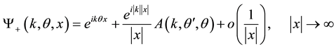(2)

where is the scattering amplitude and for

(3)

Let us also dene the solution for as

As is well known [9] :

(4)

This equation is the key to solving the inverse scattering problem, and was first used by Newton [10] [11] and Somersalo et al. [12] .

Equation (4) is equivalent to the following:

(5)

where S is a scattering operator with kernel,

The following theorem was stated in [9] :

Theorem 1. (The energy and momentum conservation laws) Let. Then, , where I is a unitary operator.

Definition 1. The set of measurable functions with norm defined by is recognized as being of Rollnik class.

As shown in [13] , is an orthonormal system of H eigenfunctions for the continuous spectrum. In addition to the continuous spectrum there are a finite number N of H negative eigenvalues, designated as with corresponding normalized eigenfunctions

where

We present Povzner’s results [13] below:

Theorem 2. (Completeness) For both an arbitrary and for H eigenfunctions, Parseval’s identity is valid.

(6)

where and are Fourier coefficients for the continuous and discrete cases.

Theorem 3. (Birman-Schwinger estimation). Let. Then, the number of discrete eigenvalues can be estimated as:

(7)

This theorem was proved in [14] .

Let us introduce the following notation:

(8)

(9)

where

We define the operators for as follows:

(10)

(11)

Consider the Riemann problem of finding a function, that is analytic in the complex plane with a cut along the real axis. Values of on the upper and lower sides of the cut are denoted and respectively. The following presents the results of [15] :

Lemma 1.

(12)

Theorem 4. Let,; then

(13)

The proof of the above follows from the classic results for the Riemann problem.

Lemma 2. Let

Then,

(14)

The proof of the above follows from the definitions of and.

Lemma 3. Let

Then,

(15)

The proof of the above again follows from the definitions of the functions and.

Lemma 4. Let Then,

(16)

The proof of the above follows from the definitions of and and Theorem 1.

Lemma 5. Let Then,

(17)

The proof of the above follows from the definitions of and and Lemma 4 and dispersions relations for analytics functions.

Definition 2. Denote by TA the set of functions with the norm

Definition 3. Denote by the set of functions such that, for any.

Lemma 6. Suppose. Then, the operator, defined on the setTA has an inverse defined on.

The proof of the above follows from the definitions of and the conditions of Lemma 6.

Lemma 7. Let, and assume that exists. Then,

(18)

The proof of the above follows from the denitions of and and Equation (4).

Lemma 8. Let, and assume that exists. Then,

(19)

where represents terms of highest order of.

The proof. Using

and (18) we get proof.

Lemma 9. Let. Then,

(20)

The lemma can be proved by substituting into Equation (1).

Lemma 10. Let, and assume that exists. Then,

(21)

The proof of the above follows from the definitions of and Lemma 7.

Lemma 11. Let. Then

The proof of the above follows from the definition of D and the unitary nature of S.

Lemma 12. Let. Then,

(22)

(23)

The proof of the above follows from the definitions of, and (1).

Lemma 13. Let, and. Then,

(24)

To prove this result, one should calculate using (18).

(25)

Using the notation that:

For

(26)

Lemma 14. Let, and. Then,

(27)

To prove this result, one should using Lemma 7.

(28)

Using Lemma 7.

Lemma 15. Let, and. Then,

(29)

(30)

To prove this result, one should calculate A using Lemma 7.

Lemma 16. Let and

Then,

(31)

A proof of this lemma can be obtained using Plancherel’s theorem.

Lemma 17. Let and

Then,

(32)

(33)

To prove this result, one should calculate.

3. Cauchy Problem for the Navier-Stokes Equation

Numerous studies of the Navier-Stokes equations have been devoted to the problem of the smoothness of its solutions. A good overview of these studies is given in [16] - [20] . The spatial differentiability of the solutions is an important factor, this controls their evolution. Obviously, differentiable solutions do not provide an effective description of turbulence. Nevertheless, the global solvability and differentiability of the solutions has not been proven, and therefore the problem of describing turbulence remains open. It is interesting to study the properties of the Fourier transform of solutions of the Navier-Stokes equations. Of particular interest is how they can be used in the description of turbulence, and whether they are differentiable. The differentiability of such Fourier transforms appears to be related to the appearance or disappearance of resonance, as this implies the absence of large energy flows from small to large harmonics, which in turn precludes the appearance of turbulence. Thus, obtaining uniform global estimations of the Fourier transform of solutions of the Navier-Stokes equations means that the principle modeling of complex flows and related calculations will be based on the Fourier transform method. The authors are continuing to research these issues in relation to a numerical weather prediction model; this paper provides a theoretical justification for this approach. Consider the Cauchy problem for the Navier-Stokes equations:

(34)

(35)

in the domain, where:

(36)

The problem defined by (34), (35), (36) has at least one weak solution in the so-called Leray-Hopf class [16] .

The following results have been proved [17] :

Theorem 5. If

(37)

there is a single generalized solution of (34), (35), (36) in the domain, , satisfying the following conditions:

(38)

Note that depends on and.

Lemma 18. Let. Then,

(39)

Our goal is to provide global estimations for the Fourier transforms of the derivatives of the solutions to the Navier-Stokes Equations (34)-(36) without requiring the initial velocity and force to be small. We obtain the following uniform time estimation.

Statement 1. The solution of (34), (35), (36) according to Theorem 5 satisfies:

(40)

where

This follows from the definition of the Fourier transform and the theory of linear differential equations.

Statement 2. The solution of (34), (35), (36) satisfies:

(41)

and the following estimations:

(42)

(43)

This expression for is obtained using div and the Fourier transform presentation.

Lemma 19. The solution of (34), (35), (36) in Theorem 5 satisfies the following inequalities:

(44)

Proof this follows from the a priory estimation of Lemma18 and conditions of Lemma 19.

Lemma 20. Let Then, the solution of (34), (35), (36) in Theorem 5 satisfies 2 the following inequalities:

(45)

Proof this follows from the a priory estimation of Lemma18 and conditions of Lemma 20.

Lemma 21. The solution of (34), (35), (36) in Theorem 5 satisfies the following inequalities:

(46)

or

(47)

Proof this follows from the a priory estimation of Lemma18, conditions of Lemma 19, the Navier-Stokes equations.

Lemma 22. The solution of (34), (35), (36) satisfies the following inequalities:

(48)

(49)

(50)

Proof this follows from the a priory estimation of Lemma 18, conditions of Lemma 22, the Navier-Stokes equations.

Lemma 23. The solution of (34), (35), (36) according to Theorem 5 satisfies, where:

(51)

Proof this follows from the a priory estimation of Lemma18, the Navier-Stokes equations.

Lemma 24.Weak solution of problem (34), (35), (36) from Theorem 5 satisfies the following inequalities:

where are limited.

Let is prove the first estimate. These inequalities

where

Proof now this follows from the a priori estimation of Lemma 18, conditions of Lemma 24, the Navier-Stokes equations.

The rest of estimates are proved similarly.

Lemma 25. Suppose that and

Then,

Proof. Using Plansherel’s theorem, we get the statement of the lemma.

This proves Lemma 25.

Lemma 26. Weak solution of problem (34), (35), (36) from Theorem 5 satisfies the following inequalities

(52)

where

Proof. From (40) we get

(53)

where

Using the notation

taking into account Holder’s inequality in I we obtain:

(53)

where and satisfies the equality. Suppose. Then

Taking into consideration the estimate I in (53), we obtain the statement of the lemma.

This proves Lemma 26.

Lemma 27. Weak solution of problem (34), (35), (36) from Theorem 5 satisfies the following inequalities

(54)

Proof. The underwritten inequalities follows from representation (40)

Let us introduce the following denotation

then

Estimate I₁ by means of

where we obtain

On applying Holder’s inequality, we get

where p, q satisfies the equality.

For we have

Inserting in to

we obtain the statement of the lemma.

This completes the proof of Lemma 27.

Lemma 28. Weak solution of problem (34), (35), (36) from Theorem 5 satisfies the following inequalities

(55)

where

Lemma 25. Let and

Then,

(56)

A proof of this lemma can be obtained using Plancherel’s theorem.

We now obtain uniform time estimations for Rollnik’s norms of the solutions of (34), (35), (36).The following (and main) goal is to obtain the same estimations for―velocity components of the Cauchy problem for the Navier-Stokes equations.

Let’s consider the influence of the following large scale transformations in Navier-Stokes’ equation on

Statement 3. Let

Proof. By the definitions and we have

This proves Statement 3.

Theorem 6. Let

and

Then, there exists a unique generalized solution of (34), (35), (36) satisfying the following inequality:

where the value of depends only on the conditions of the theorem.

Proof. It suffices to obtain uniform estimates of the maximum velocity components, which obviously follow from because uniform estimates allow us to extend the local existence and uniqueness theorem over the interval in which they are valid. To estimate the velocity components, Lemma 22 can be used:

Using Lemmas (25)-(29) for

we can obtain where is the amplitude of potential and. That is, discrete solutions are not significant in proving the theorem, so its assertion follows the conditions of Theorem 6, which defines uniform time estimations for the maximum values of the velocity components.

(57)

Theorem 6 asserts the global solvability and uniqueness of the Cauchy problem for the Navier-Stokes equations.

Theorem 7. Let

(58)

Then, there exists and

(59)

Proof. A proof of this lemma can be obtained using and uniform estimates.

Theorem 7 describes the loss of smoothness of classical solutions for the Navier-Stokes equations.

Theorem 7 describes the time blow up of the classical solutions for the Navier-Stokes equations arises, and complements the results of Terence Tao [17] .

4. Conclusion

New uniform global estimations of solutions of the Navier-Stokes equations indicate that the principle modeling of complex flows and related calculations can be based on the Fourier transform method.

Acknowledgements

We are grateful to the Ministry of Education and Science of the Republic of Kazakhstan for a grant, and to the System Research “'Factor” Company for combining our efforts in this project.

The work was performed as part of an international project, “Joint Kazakh-Indian studies of the influence of anthropogenic factors on atmospheric phenomena on the basis of numerical weather prediction models WRF (Weather Research and Forecasting)”, commissioned by the Ministry of Education and Science of the Republic of Kazakhstan.

References

- Fefferman, C.L. (2006) Existence and Smoothness of the Navier-Stokes Equation. The Millennium Prize Problems, Clay Mathematics Institute, Cambridge, 57-67.
- Durmagambetov, A.A. and Fazilova, L.S. (2013) Global Estimation of the Cauchy Problem Solutions’ Fourier Transform Derivatives for the Navier-Stokes Equation. International Journal of Modern Nonlinear Theory and Application, 2, 232-234. http://www.scirp.org/journal/IJMNTA/
- Durmagambetov, A.A. and Fazilova, L.S. (2014) Global Estimation of the Cauchy Problem Solutions’ the Navier- Stokes Equation. Journal of Applied Mathematics and Physics, 2, 17-25. http://www.scirp.org/journal/JAMP/
- Durmagambetov, A.A. and Fazilova, L.S. (2014) Existence and Blowup Behavior of Global Strong Solutions Navier- Stokes. International Journal of Engineering Science and Innovative Technology, 3, 679-687. http://ijesit.com/archivedescription.php?id=16
- Russell, J.S. (1844) Report on Wave. Report of the Fourteenth Meeting of the British Association for the Advancement of Science, York, Plates XLVII-LVII, 90-311.
- Russell, J.S. (1838) Report of the Committee on Waves. Report of the 7th Meeting of British Association for the Advancement of Science, John Murray, London, 417-496.
- Ablowitz, M.J. and Segur, H. (1981) Solitons and the Inverse Scattering Transform. SIAM, 435-436.
- Zabusky, N.J. and Kruskal, M.D. (1965) Interaction of Solitons in a Collisionless Plasma and the Recurrence of Initial States. Physical Review Letters, 15, 240-243. http://dx.doi.org/10.1103/PhysRevLett.15.240
- Faddeev, L.D. (1974) The Inverse Problem in the Quantum Theory of Scattering II. Itogi Nauki i Tekhniki, Seriya Sovremennye Problemy Matematiki, Fundamental’nye Napravleniya, VINITI, Moscow, 93-180.
- Newton, R.G. (1979) New Result on the Inverse Scattering Problem in Three Dimensions. Physical Review Letters, 43, 541-542. http://dx.doi.org/10.1103/PhysRevLett.43.541
- Newton, R.G. (1980) Inverse Scattering. II. Three Dimensions. Journal of Mathematical Physics, 21, 1698-1715. http://dx.doi.org/10.1063/1.524637
- Somersalo, E., et al. (1988) Inverse Scattering Problem for the Schrodinger’s Equation in Three Dimensions: Connections between Exact and Approximate Methods. Journal of Mathematical Physics, 21, 1698-1715.
- Povzner, A.Y. (1953) On the Expansion of Arbitrary Functions in Characteristic Functions of the Operator. Russian, Sbornik Mathematics, 32, 56-109.
- Birman, M.S. (1961) On the Spectrum of Singular Boundary-Value Problems. Russian, Sbornik Mathematics, 55, 74- 125.
- Poincare, H. (1910) Lecons de mecanique celeste, t. Math. & Phys. Papers, 4, 141-148.
- Leray, J. (1934). Sur le mouvement d’un liquide visqueux emplissant l’espace. Acta Mathematica, 63, 193-248. http://dx.doi.org/10.1007/BF02547354
- Ladyzhenskaya, O.A. (1970) Mathematics Problems of Viscous Incondensable Liquid Dynamics. Science, 288.
- Solonnikov, V.A. (1964) Estimates Solving Nonstationary Linearized Systems of Navier-Stokes’ Equations. Transactions Academy of Sciences USSR, 70, 213-317.
- Huang, X., Li, J. and Wang, Y. (2013) Serrin-Type Blowup Criterion for Full Compressible Navier-Stokes System. Archive for Rational Mechanics and Analysis, 207, 303-316. http://dx.doi.org/10.1007/s00205-012-0577-5
- Tao, T. (2014) Finite Time Blowup for an Averaged Three-Dimensional Navier-Stokes Equation.