Engineering
Vol.4 No.12A(2012), Article ID:26074,8 pages DOI:10.4236/eng.2012.412A120
Migrated Exploding Reflectors in Evaluation of Finite Difference Solution for Inhomogeneous Seismic Models
1R&D Department, Dana Geophysics Co., Tehran, Iran
2Institute of Geophysics, University of Tehran, Tehran, Iran
Email: nejati.maryam@danaenergy.ir, hashemy@ut.ac.ir
Received August 15, 2012; revised September 24, 2012; accepted October 4, 2012
Keywords: Finite Difference Method; Seismic Modeling; Migration; Exploding Reflector; Structural Similarity Index
ABSTRACT
Earth is inhomogeneous, which means its elastic characteristics change with depth. The seismic method employs the propagation of waves throughout the earth to locate different structures and stratigraphy. Understanding the wave propagation is an important matter in exploration seismology; therefore modeling of seismic wave is an important tool. To validate the interpreted earth model out of the seismic data, seismic synthetic seismograms should be generated in a process named “seismic forward modeling”. Finite difference method is used as one of the most common numerical modeling techniques. In this paper the accuracy of finite difference method in seismic section modeling is explored on different modeled data set of heterogeneous earth. It is shown that finite difference method completes with migration to reposition the events in their correct location. Two different migration methods are used and various velocities are also tested to determine an appropriate migration velocity. Finally the validly of finite difference modeling is examined using a 2D structural similarity index technique.
1. Introduction
The seismic method employs the propagation of waves throughout the earth to locate deposits such as hydrocarbons, reservoirs, ores and etc. Earth is inhomogeneous, which means its elastic properties varies with depth and changes from a region to the nearby one. Although the variation may be gradual, there are distinct discontinuities that separate media with different densities and elastic coefficients producing reflection boundaries. In propagation of seismic waves from one medium to another with different properties, some part of energy is reflected back to the first medium and the other portion is transmitted into the second one. The strength of reflection depends on the acoustic impedance contrast of two mediums, whereas acoustic impedance is the product of medium velocity and density. Relationship between the stress and displacement vectors of two sides of the interface is a deterministic factor in portioning of energy. This was first developed and formulated by Zoeppritz [1] in the form of amplitudes and Knott [2] as the potential functions.
One of the basic techniques to validate the interpreted earth model out of the seismic data is to generate seismic synthetic seismograms. This is mainly named as the forward modeling procedure. Since understanding the wave propagation is a fundamental issue in exploration seismology, modeling of seismic wave would be a valuable tool. Seismic wave equations, used to describe seismic wave propagation in the subsurface, are typically partial differential equations containing spatial and temporal derivatives. There are different numerical methods of seismic modeling such as ray tracing methods and wave equation methods including Kirchhoff integration, finite difference (FD), finite element (FE) and etc. Wave equation numerical method can extract the information of both travel time and amplitude of seismic wave and can explain wave propagation in complicated medium. Finite difference method is one of the most common modeling methods [3-6]. This method is theoretically based on a Taylor series representation of the wave field resulting in a formulation for numerical estimation of the derivatives appearing in the wave equation.
One straightforward application of seismic modeling is the development of models to address problems of structure and stratigraphy during the interpretation of seismic data. This helps an interpreter relate the modeled seismic response generated from a hypothesized geologic model with the seismic data being interpreted. Understanding the spatial organization of subsurface structures such as dip layers, fault, thrust, reef, salt dome, channels, traps and etc., and their response to seismic wave propagation is essential for interpreters which help them to recognize these structures better in seismic sections.
In this paper, the accuracy of solving seismic wave in different heterogeneous model using finite difference scheme is studied and the validly of modeling is investigated using a 2D similarity evaluation technique.
2. Finite Difference Solver for Seismic Wave Equation
Scalar 2D seismic wave equation in Cartesian coordinate system is defined by,
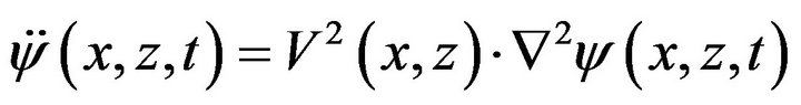 (1)
(1)
Here  is devoted for seismic wavefield in three dimensions,
  is the seismic velocity in 2D heterogeneous earth model. Using second-order time derivatives, one can predict the value of
  in the next samples without analytically solving Equation (1) as,
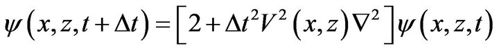 (2)
(2)
The main idea behind the FD method is to compute the wave field  at a discrete set of closely-spaced grid points
 , with
  by approximating the derivatives occurring in the equation of motion with finite difference formulas, and recursively solving the resulting difference equation. Different orders are defined for solving Equation (2) based on the length of forward and backward filter.
3. Exploding Reflector Model
In surface seismic acquisition both receivers and source points are placed on the earth. This mimics the meaning of two-way travel time. Unlike this practical way, one numerical simplification when post-stack velocity files are accessed is to assume that sources are placed on the reflection boundaries. At time zero, the reflectors all explode with strength proportional to their normal-incidence reflection coefficients. The resulting wave field, at the instant of zero time morphologically identical to the reflectors and time, will propagate along normal incidence ray paths. Figure 1 shows a schematic view of
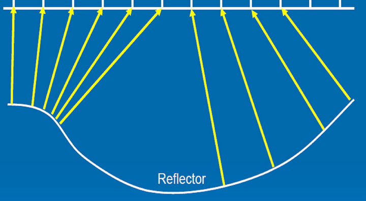
Figure 1. An exploding reflector model, theoretically sources are placed on the reflector.
exploding reflector shooting in a programming environment. The essence of this technique together with implementing this method in Matlab is discussed [7-9].
4. Seismic Synthetic Modeling
To examine the effect of finite difference method in seismic forward modeling, four different velocity models are generated. They are mainly a channel, an anticline, a thrust and a known model named Marmusi respectively. To explore the functionality of finite difference method in modeling seismic responses of complex geological structures, exploding reflectors concept is used.
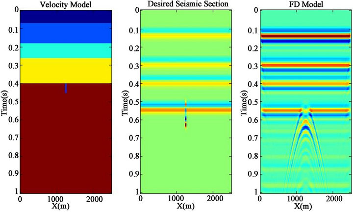
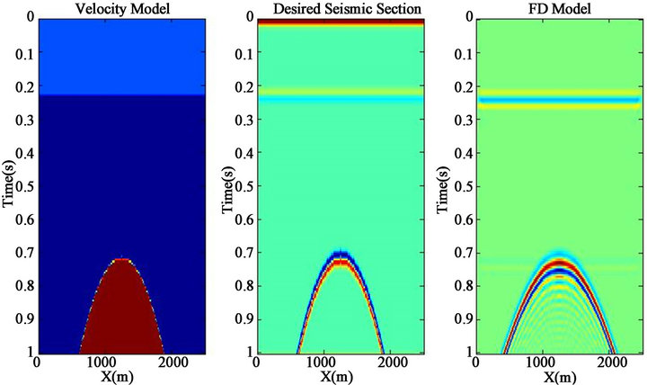
Figure 2(a) shows the velocity model of a small-buried channel in a layered medium. The width and depth of the channel are 20 m and 50 m respectively. Survey design parameters are consisting of some important factors like receiver interval (RI), number of time samples and central frequency of the wavelet (f). To generate a seismic section of this model, RI is chosen as 5 meters (i.e. the channel is 4 samples in X and 10 samples in time) and a zero phase wavelet with the f = 30 Hz was convolved with the velocity-time model. Prior to this, the velocity matrix shall be converted from depth to time by using the relationship between depth and vertical travel time. This is the model described as the input to the convolutional model theory (Figure 2(b)). It states that a given reflectivity is the convolution result of acoustic impedance (velocity when densities are constant) and used wavelet.
The modeling will be completed using finite difference operator based on exploding reflector theory, which assumes that shot points are placed on the reflectors. Input parameters in the module are the temporal and spatial sample sizes, the maximum record time, the velocity matrix, the receiver positions, the wavelet and the desired Laplacian (forth order). Figure 2(c) shows the “FD model” relevant to the velocity section using the forth order Laplacian operator. The 30 Hz frequency wavelet is designed to remove some of the effects of the artificial grid dispersion.
The channel produces an extensive diffraction pattern showing scattered energy over the entire model. To eliminate these patterns, seismic migration is needed. In exploration seismology, migration refers to a multichannel processing step that spatially re-position events and progress focusing. Before migration, seismic data is usually displayed with traces plotted at the surface location of the receivers and with a vertical time axis. This means that dipping reflections are systematically mispositioned in the lateral coordinate and the vertical time axis needs a transformation to depth. Additionally, migration algorithms perform amplitude and phase adjustments that are planned to correct for the effects of the spreading or convergence of ray paths as wave propagate. There are many approaches for migration including
 (a) (b) (c)
Figure 2. (a) Velocity model of a buried channel (dark blue); (b) Desired seismic section; (c) FD model before migration.
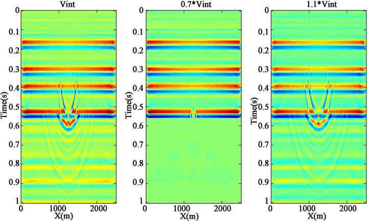
Kirchhoff, finite difference, frequency-domain and phaseshift methods [10]. The Kirchhoff method migrates the data by searching for diffractions and moving all energy along the diffraction curve to its apex so it was used in channel model to remove diffractions. An important point that should be considered is that the migration velocity is the velocity required to best migrate the seismic data related to the true interval velocity and is not the stacking velocity. For assessing the effect of selecting correct velocity in migration, 3 different velocity matrixes selected to be used for migration as shown in Figure 3. In Figure 3(a), the velocity matrix is exactly the same used in the FD model, while in Figures 3(b) and 3(c) it is 0.7 of the velocity matrix and 1.1 of the velocity matrix respectively. It is obvious that the Figure 3(b) has the best result in migration and all the diffraction patterns are removed perfectly and energy is collapsed to the channel location.
As a slightly more complicated example, the response of an anticline beneath a layer as shown in Figure 4(a) was explored that will be useful in examining in seismic response modeling. In Figure 4(b) the seismic section of this model obtained from convolution of a 30 Hz zero phase wavelet with the velocity-time section is shown. The fourth-order Laplacian exploding reflector seismogram is shown in Figure 4(c) that was created with a spatial grid size of 5 m.
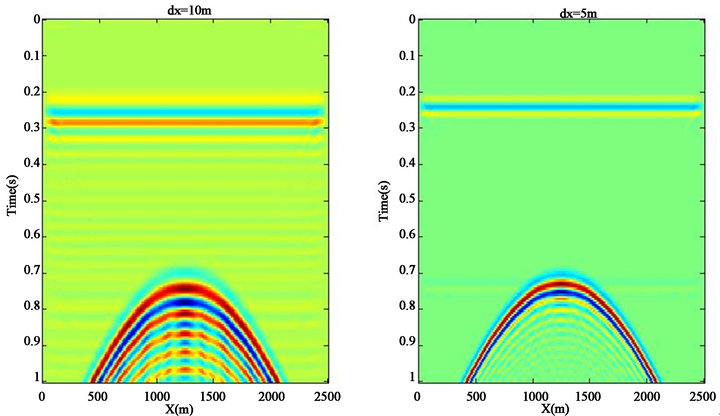
While working with finite difference method for seismic modeling, it should be considered how to choose the parameters to increase the precision. For example, as shown in Figure 5(a), selecting the spatial grid size of 10 m will cause series of reverberations following the primary response but with recreating the model with a finer spatial grid size (5 m) the reverberations will be disappeared (Figure 2(b)). Therefore for an accurate modeling with finite difference method optimizing different parameters is needed and hence the computation time will increase. Comparing Figures 4(b) and 4(c), the anticline appears broader than its true shape. In fact in an unmigrated section, dipping reflections have apparent dips less than the dip of the reflectors and apparent lengths greater than the actual lengths of the reflectors. So anticline seems wider.
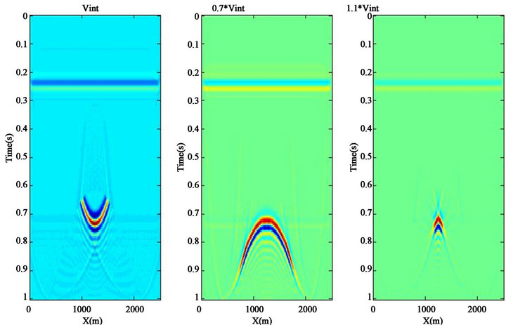
To counteract this problem Kirchhoff migration method was used with three different velocities including the interval velocity matrix used in the FD model, 0.5 of the velocity matrix and 0.8 of the velocity matrix respecttively as shown in Figure 6. Clearly the best outcome is related to the Figure 6(b) that the anticline looks smaller than the unmigrated section (Figure 6(c)) similar to the desired section (Figure 6(b)).
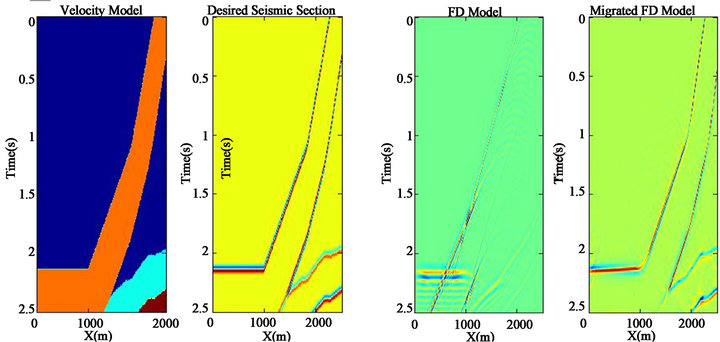
In next step a complex thrust structure (kind of reverse fault) is considered for this analysis. Figure 7(a) represents velocity depth model for the thrust structure. The desired seismic section resulting from the convolution of the 30 Hz zero phase wavelet with the velocity time model is shown in Figure 7(b) and the fourth-order finite difference model of the thrust model is displayed in Figure 7(c). In this model there is steep dip that it is not clear and mispositioned in the FD model and needs to be migrated. Figure 7(d) shows the FD model after migration with phase-shift method. Phase-shift is one of the migration methods, which is a recursive approach that uses a series of constant velocity extrapolations to build a v(z) migration. The velocity matrix for migration was chose 0.5 of the interval velocity matrix that could migrate the section perfectly in comparison with Figure 7(b), the desired section.
 (a) (b) (c)
Figure 3. (a) Migrated section using 100% of interval velocity of a buried channel; (b) Migrated section using 70% of interval velocity of a buried channel; (c) Migrated section using 110% of interval velocity of a buried channel.
 (a) (b) (c)
Figure 4. (a) Velocity model of an anticline (dark red); (b) Desired seismic section; (c) FD model before migration.
To examining finite difference method in seismic modeling, a complicated model named Marmousi is studied as the last model (Figure 8). The Institute Français du Pétrole (IFP) created the Marmousi model in 1988. The geometry of this model is based on a profile through the North Quenguela trough in the Cuanza basin. The geometry and velocity model were created to produce complex seismic data, which has come be a sort of industry standard and almost classic dataset. The Marmousi model contains 158 horizontally layered horizons.
The model sits under approximately 32 m of water and is 9.2 km in length and 3 km in depth.
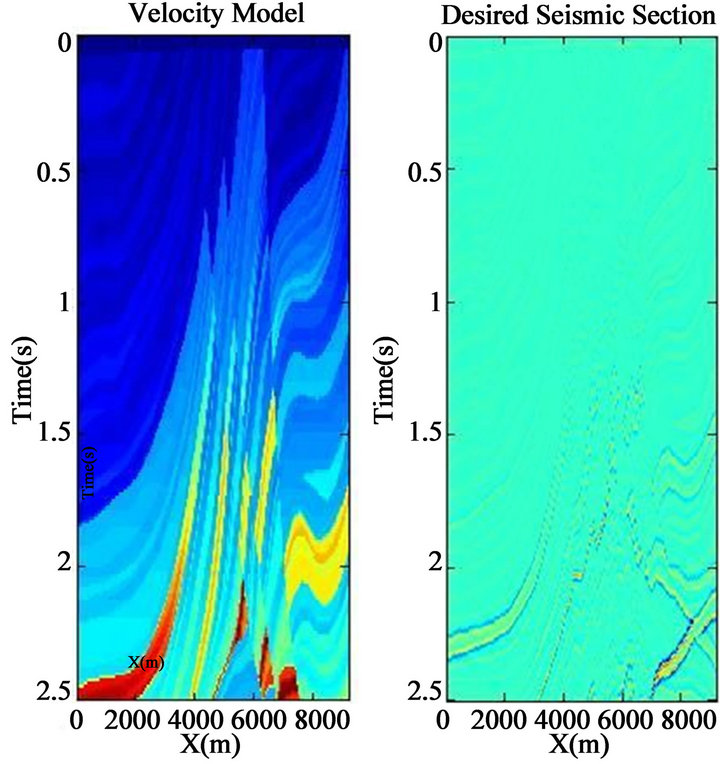
Part of Marmousi model as shown in Figure 9(a) was used here for the finite difference analysis. Figure 9(b) shows the desired seismic section of convolving Marmousi time model with the 30 Hz frequency zero phase
 (a) (b)
Figure 5. (a) FD model of an anticline with grid size of 10 m; (b) FD model of an anticline with grid size of 5 m. Undesired reverberation is visible in larger grid size model due to numerical errors.
 (a) (b) (c)
Figure 6. (a) Migrated section using 100% of interval velocity of anticline; (b) Migrated section using 50% of interval velocity of anticline; (c) Migrated section using 80% of Interval velocity of anticline.
 (a) (b) (c) (d)
Figure 7. (a) Velocity model of a thrust; (b) Desired seismic section; (c) FD model before migration; (d) Migrated section using 50% of interval velocity of thrust.
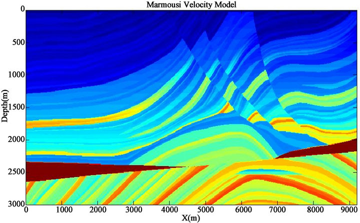
Figure 8. Marmousi velocity model.
wavelet. The forth order Laplacian finite difference equation of Marmousi model is displayed in Figure 9(c) and the migrated FD section using phase-shift migration method can be seen in Figure 9 (d).
To estimate how accurately the finite difference equation can model the seismic section the structural similarity (SSIM) index between the migrated finite difference model and desired seismic section is computed for all four geological structures in this paper (Table 1). SSIM [11] is a method for measuring the similarity between two images. If two images are exactly the same then SSIM will be reported as one.
5. Discussion and Conclusion
Examining four different geological models, and apply-
 (a)
(a)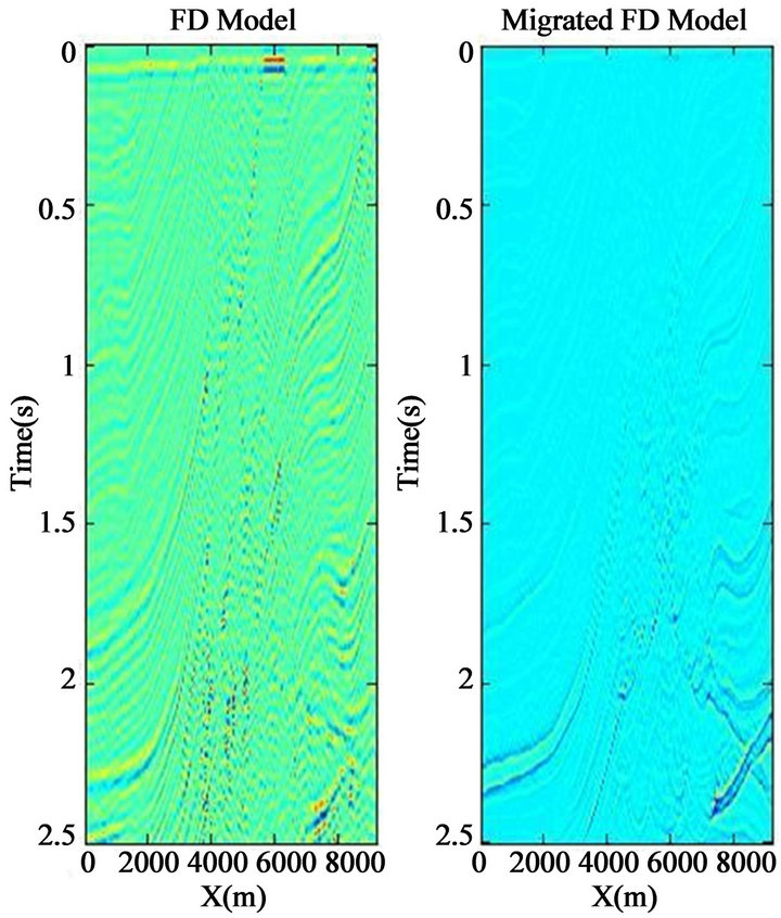 (b)
(b)
Figure 9. (a) Marmousi velocity model; (b) Desired seismic section; (c) FD model before migration; (d) Migrated section using 50% of Interval velocity of thrust.
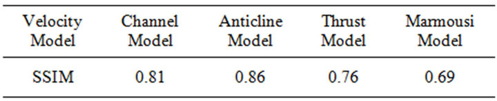
Table 1. Structural similarity index showing degree of coherency between desired output and FD model after migration. Larger values are relevant to better jobs of FD + migration.
ing finite difference method for exploding reflectors, it was seen that the FD equation can model the seismic section suitably. It should be noted that choosing parameters for the finite difference modeling is an important issue that affects the results. Additionally, migration is necessary after finite difference to position the events in their true location. Since migration velocity is different from stacking velocity, determining the appropriate velocity, is very important for true migration. Furthermore, there are different methods for migration that each of them has its own advantages depending on the seismic data features such as dip of events and signal to noise ratio. It is even found for a very complex model (Marmousi) that a classic post-stack migration does not yield to a high SSIM. This amplifies need to have pre-stack depth migration algorithm that consequently limits the use of the proposed scheme for very complicated areas. When degree of model inhomogeneity increases, finite difference or any other numerical methods shall be run on pre-stack domain. Considering these issues this forward modeling problem can act as a foundation for understanding seismic wave propagation and it can be used as a tool for the seismic imaging and inversion problems.
REFERENCES
- K. Zoeppritz, “Erdbebenwellen VII. VIIb. Über Reflexion und Durchgang Seismischer Wellen durch Unstetigkeitsflächen. Nachrichten von der Königlichen Gesellschaft der Wissenschaften zu Göttingen,” Mathematisch-Physikalische Klasse, 1919, pp. 66-84.
- R. E. Sheriff and L. P. Geldart, “Exploration Seismology,” 2nd Edition, Cambridge University Press, Cambridge, 1995. doi:10.1017/CBO9781139168359
- M. Zaitian, “Seismic Imaging Technology: The Finite Difference Migration,” China Petroleum Industry Press, Beijing, 1989.
- J. E. Vidale, “Finite-Difference Calculation of Traveltimes in Three Dimensions,” Geophysics, Vol. 55, No. 5, 1990, pp. 521-526. doi:10.1190/1.1442863
- R. T. Coates and M. Schoenberg, “Finite-Difference Modeling of Faults and Fractures,” Geophysics, Vol. 60, 1995, pp. 1514-1526. doi:10.1190/1.1443884
- A. Pitarka, “3D Elastic Finite-Difference Modeling of Seismic Motion Using Staggered Grids with Nonuniform Spacing,” Bulletin of the Seismological Society of America, Vol. 89, 1999, pp. 54-68.
- C. F. Youzwishen and G. F. Margrave, “Finite Difference Modelling of Acoustic Waves in Matlab,” Crewes Report, Vol. 11, 1999, pp. 1-19.
- J. M. Carcione, G. Böhm and A. Marchetti, “Simulation of a CMP Seismic Section,” Journal of Seismic Exploration, Vol. 3, 1994, pp. 381-396.
- D. Loewenthal, L. Lu, R. Roberson and J. W. C. Sherwood, “The Wave Equation Applied to Migration,” Geophysical Prospecting, Vol. 24, 1976, pp. 380-399.
- J. F. Claerbout, “Basic Earth Imaging: Stanford Exploration Project,” Preliminary, 1993. http://sepwww.stanford.edu/sep/prof/index.html
- Z. Wang, A. C. Bovik, H. R. Sheikh and E. P. Simoncelli, “Image Quality Assessment: From Error Visibility to Structural Similarity,” IEEE Transactions on Image Processing, Vol. 13, No. 4, 2004, pp. 600-612. doi:10.1109/TIP.2003.819861