Applied Mathematics
Vol.09 No.02(2018), Article ID:82707,15 pages
10.4236/am.2018.92010
Cross-Correlation of Station-to-Station Free Surface Elevation Time Series for Breaking Water Waves
Raphael Mukaro
School of Mathematical and Physical Sciences, Department of Physics & Electronics, North West University, Mafikeng Campus, Mmabatho, South Africa

Copyright © 2018 by author and Scientific Research Publishing Inc.
This work is licensed under the Creative Commons Attribution International License (CC BY 4.0).
http://creativecommons.org/licenses/by/4.0/


Received: December 18, 2017; Accepted: February 25, 2018; Published: February 28, 2018
ABSTRACT
Free surface elevation time series of breaking water waves were measured in a laboratory flume. This was done in order to analyze changes in wave characteristics as the waves propagated from deep water to the shore. A pair of parallel-wire capacitive wave gages was used to simultaneously measure free surface elevations at different positions along the flume. One gage was kept fixed near the wave generator to provide a reference while the other was moved in steps of 0.1 m in the vicinity of the break point. Data from these two wave gages measured at the same time constitute station-to-station free surface elevation time series. Fast Fourier Transform (FFT) based cross-correlation techniques were employed to determine the time lag between each pair of the time series. The time lag was used to compute the phase shift between the reference wave gage and that at various points along the flume. Phase differences between two points spaced 0.1 m apart were used to calculate local mean wave phase velocity for a point that lies in the middle. Results show that moving from deep water to shallow water, the measured mean phase velocity decreases almost linearly from about 1.75 m/s to about 1.50 m/s at the break point. Just after the break point, wave phase velocity abruptly increases to a maximum value of 1.87 m/s observed at a position 30 cm downstream of the break point. Thereafter, the phase velocity decreases, reaching a minimum of about 1.30 m/s.
Keywords:
Turbulence, Plunging Breaker, Time Series, Cross-Correlation, Relative Phase, Phase Velocity

1. Introduction
Water waves that develop on the open sea propagate towards the shore, undergo a series of transformations, the description of which presents both theoretical and experimental challenges [1] . Flow theory quite well predicts the physics of wave shoaling over a slope up to and into the early stages of breaking, but the same cannot be said after the break point [2] . Beginning offshore where the water depth is sufficiently deep and constant, water waves are observed to be symmetric with respect to the wave crest before they begin to deform due to interactions with the bathymetry [3] . As they propagate from deep water to shallow water of the surf zone beach slope, they also slow down and grow taller. The change in wave height due to varying water depths is called wave shoaling. The phenomenon of wave shoaling is directly related to bottom slope where on a gentler slope shoaling is greater as compared to a sufficiently steep slope [2] . At a depth of half its wave length, rounded waves start to rise and their crests become shorter while their troughs lengthen. Although their period (frequency) stays the same, the waves slow down and their overall wavelength shortens. This implies that phase velocity varies as waves propagate and break along the flume. This phase velocity is one of the important parameters in wave mechanics. Due to shoaling, asymmetry of the wave and the wave height continues to increase until at some critical point (break point) where the wave becomes unstable and collapses. This critical point depends on the wave height and also the beach slope. Breaking of waves is characterized by top of the crest falling onto the front face of the wave, forming a body of fluid, called the roller that rides on the wave front. This process entraps considerable amount of air which bursts into small bubbles, and results in energy dissipation and the transfer of momentum to currents. The roller interacts with the fluid below it in a complicated way, exchanging energy and momentum in the process. The roller will eventually dissipate and be completely absorbed by the wave. However, if breaking continues to occur, the roller will be sustained for the greater portion of the surf zone. Thus there will be a shoreward mass transport occurring above the trough level.
Wave theory is essential in order to predict and analyze changes in the characteristics of a wave as it propagates from the deep water to the shore. Such theories and empirical formulae have been proposed for the calculation of wave phase velocity and the prediction of breaking as a result of wave shoaling. In an early investigation, Suhayda & Petrigrew [4] used a photographic technique involving calibrated wave poles placed across the breaker zone to measure wave phase speed. The average wave crest speed was approximated by measuring the distance a particular wave crest had moved over the interval of time and then compared to solitary theory. Maximum discrepancies were observed at the break point, where measured speeds were 20% greater than those predicted by solitary theory, and in the mid surf zone, where measured values were ~20% less than the predicted values. Errors in the calculation were attributed to problems in visually determining the crest of the wave and to the fact that the speed of the crest does not represent the speed of the wave as a whole. Stansell & MacFarlane [5] used a series of wave guides 0.1 m apart and fitted the crest position data to a second order polynomial, differentiating the equation to determine wave velocity. Yoo et al. [6] measured the celerity of incident waves obtained from oblique video imagery in the nearshore. Wave phase velocity was computed along a cross-shore transect from the wave crest tracks extracted by a Radon transform-based line detection method. The phase velocity from the nearshore video imagery was observed to be larger than the linear wave celerity computed from the measured water depths over the entire surf zone. Lippmann & Holman [7] tested the capability of video data analysis for estimation of phase speed and wave angle of individual breaking waves. Phase speeds and wave angles were calculated using pixel intensity time series collected with a 4-m-wide square array. Measured wave phase velocities exceeded linear theory by up to 20%, suggesting some amplitude dispersion. Tissier et al. [8] performed field measurements and non-linear prediction of wave phase velocity in the surf zone. Their work is based on a unique dataset inside the surf zone, including data for very shallow water and very strong nonlinearities. They analyzed and quantified the effects of non-linearities and evaluated the predictive ability of several non-linear celerity predictors for high-energy wave conditions. Using cross-correlation techniques, they accurately determined the time lag between two wave time series recorded by two closely space wave gages, to obtain an accurate local velocity prediction.
2. Statement of the Problem
In this work carefully planned wave phase velocity measurements under known and controlled laboratory conditions are to be conducted in wave flume. Measurements were taken in the vicinity of the break point in laboratory plunging wave flow. The aim is to get some indication of the accuracy of small-amplitude wave theory in predicting the transformation of monochromatic two-dimensional waves as they propagated from intermediate to shallow water depths. Free surface elevation time series measurements were to be made at several positions along the flume using a pair of capacitive wave gages, where one was fixed (reference) and the other mobile. The measurements are to be recorded simultaneously on the computer at each position. Time lags at these positions will be estimated by cross correlating each mobile gage time series with that of the reference wave gage, taken at the same time. This should allow for the computation of relative wave phase along the flume. Local wave phase velocity for points 0.1 m apart will then be computed from relative phases and compared with results from linear shallow water approximation, . These well-controlled laboratory experiments are necessary as they provide prior information required in model experiments involving turbulent flows and computational fluid dynamics models. As pointed out by Kimmoun & Branger [9] results from this study may also be useful for calibrating wave models developed using computational fluid dynamics.
3. Propagating Wave Parameters
A wave that propagates across a surface as a train of crests and troughs is called a progressive wave. Figure 1 shows a schematic of a progressive two-dimensional sinusoidal wave propagating in the positive x direction and defines the significant parameters of this periodic wave. x, y, and z axes form a right-handed coordinate system with the positive x-axis pointing in the direction of wave propagation. The positive y direction (not shown) is into the plane of the page. The still water line (SWL) is the level of the water in the absence of waves, corresponding to elevation . The distance between the bed and the SWL, called the still water depth, is represented by d, so that the bed is at . represents the displacement of the water surface relative to the SWL, L is the wavelength and H is the height or amplitude of the wave.
For such a wave propagating in the positive x-direction, at a distance x at time t is given by:
(1)
where is the wave amplitude, , is the frequency of the
wave, and is the wave number. Equation (1) is the linear wave equation which is reasonable only for low amplitude waves. For increasing wave amplitude, the surface profile becomes vertically asymmetric with a more peaked wave crest and a flatter wave trough [10] .
Phase velocity of such a wave is the speed at which the phase of a wave propagates and is considered one of the most important parameters for propagating waves. Phase velocity is often predicted using linear shallow water theory given by [8] [11] [12] as: , where g is the acceleration due to gravity and h is the local water height. The expression implies that waves of constant period slow down as they enter shallow water and is correct only for very short depths [11] . This process of slowing down is called shoaling, and leads to steepening of the wave that leads to breaking.
4. Experimental Setup and Procedures
Experiments were conducted in a rectangular, glass-walled flume at the Coastal and Hydraulics Engineering Laboratory located at the Council for Scientific and
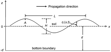
Figure 1. Sketch defining coordinate axes and wave parameters for a progressive wave propagating in the positive x direction.
Industrial Research (CSIR) in Stellenbosch, South Africa. The flume is approximately 20 m long, 0.75 m wide and has a gentle beach slope of 1:20 which was chosen in order to get a long enough surf zone length over which measurements of wave parameters could later be conducted. A 1:20 (height: length) beach slope has also been used as the standard slope by numerous researchers in similar studies [13] [14] . The flume was filled with water to a depth of about 62 cm. Regular 0.4 Hz two-dimensional waves having a wave height of 12 cm in the flat section of the flume were generated by a hydraulically driven, computer-controlled piston type wave maker manufactured by H. R. Wallingford [15] . An offshore water depth of 62 cm was set and monochromatic waves with period T = 2.5 s generated. The incident wave height was H = 12 cm. This resulted in plunging waves that broke at a distance of about 4.0 m from the still water mark on the beach. Figure 2 shows the schematic view of the flume giving overall dimensions, showing the sloping bottom and the coordinate system that is used. It illustrates characteristic regions of the flume, giving overall dimensions in addition to showing the sloping bottom and the coordinate system used. Coordinate x is directed parallel to the mean flow, and is conventionally established as positive if oriented onshore, with x = 0 at the intersection of the still water line and the beach flow, a point 1.6.0 m from the break point towards the shore. y is perpendicular to the side wall so that the y-axis is set parallel to the shore with y = 0 at a lateral point 10 cm from the flume wall of the tank. z is the vertical coordinate, conventionally established as positive if oriented upward. The z-axis is defined normal to the beach, with z = 0 at the SWL and increasing in the upward direction. The origin is at the intersection of the beach slope and the still water level. With this convention, it must be noted that horizontal distances measured along the flume will be negative for positions away from the shore, towards the wave maker.
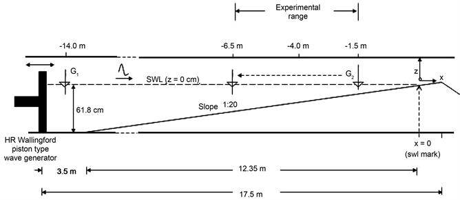
Figure 2. Side-view schematic of the wave flume (not drawn to scale) showing structure, dimensions and the reference frame used.
The time series of surface elevations were simultaneously recorded at various water depths along the beach. Instantaneous water levels were measured using a pair of parallel-wire capacitance-type wave gages, model WG-50, manufactured by RBR Ltd. The wave gages consisted of a 1 mm wire pair, which were rigidly mounted on stainless steel frames. Each wave gage was connected to an electronic circuit which consisted of two oscillators, one of fixed frequency and the other made variable by means of the changing capacitance of the probe due to changes in water level. The difference in frequency was transmitted to a frequency-to-voltage converter which provided a D.C voltage linearly proportional to the frequency difference. The wave gages were initially calibrated with no wave running in the flume. The wave gage manufacturer specifies a response time of 2 ms for a step change in water level. This more than satisfies our requirement of using 2.5 s period waves. The wave gages have an error of about 0.56% over the wave height range used. This translates to an error of approximately 0.12 cm for a maximum displacement of 21 cm of the water level, which is a typical maximum wave height at the break point in the present experiment.
The waves were allowed to run for approximately 30 minutes to ensure parameters such as the position of the break point and currents, have stabilized. Wave gage , fixed near the generator at acted as a reference, and the other , initially placed at , were used to simultaneously measure free surface elevations at several positions along the flume. A computer driven data acquisition system sampled the wave gages at 50 Hz through the WG-50 interfaces and signal conditioning circuits. Then gage was moved 10 cm towards the generator to a new position and the two sampled again. This process was repeated until a total distance of 5 m spanning the breaking and pre-breaking region was covered. Figure 3 shows a schematic of the wave generator control and data acquisition systems. The wave generator consists of a servo-driven piston paddle, a servo control unit and a computer for preprogramming the desired wave heights and frequency. Characteristics of the desired wave are first entered on the wave maker computer. The computer drives the servo controller that is
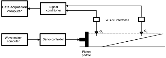
Figure 3. Block diagram showing the two wave gages connected to a data acquisition computer.
connected to a piston paddle to generate the specified waves. After the waves in the flume have stabilized, the data acquisition computer simultaneously samples the two wave gages at predetermined times.
5. Results
Free surface elevation measurements were made for regular 0.4 Hz plunging water waves with a wave height of 12 cm as it propagated and broke on a 1:20 laboratory beach slope. The flow had a Reynolds number of about 30,000 and the break point for this flow was at about 4.0 m from the beach. A computerized measurement system was used to measure discrete time series of surface elevation measurements equally spaced in time as shown in Figure 4. If the sampling frequency is , then the time interval between two succeeding points is . The total number of samples corresponding to the sample duration T is . Thus we obtain a discrete time series of surface elevation . With a sampling frequency of a reading every 0.02 s (50 Hz), there are 125 samples over a wave period of 2.5 s and a total of 6000 over a test time of 120 s. Thus 6000 samples contained approximately 48 wave cycles. Each wave gage probe contributed 6000 samples. Data sampled from the gages at each position were saved in a single text file on the computer. Table 1 shows characteristic parameters relating to free surface water level measurements, wave height and wave velocity calculations.
is the frequency of the wave, is the sampling frequency, is the total sampling time, is the number of samples captured per period of the wave, is the sample size in 120 s and is the number of full waves in the time record.
5.1. Water Level Time Series
Figure 5 shows time series of the free surface elevations, , measured at two different positions b) just before the break point and c) after the break point. Measured relative to the reference wave gage time series a). These were measured at different times. As already mentioned, although the wave gages were sampled for 120 s, in Figure 5 only the first 20 s of the time series is shown. In deep water, the waveform is close to a sinusoidal. As the wave shoals, the
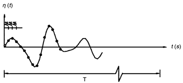
Figure 4. Discrete sampling of free surface elevation at regular intervals.

Table 1. Parameters for free surface elevation measurements and phase velocity calculation.

Figure 5. Time series of free surface elevations over a 20 s record measured simultaneously by the two wave gages at two different times, (a) -near wave generator at ( ), (b) -at the break point at ( ) and (c) -after the break point at ( ).
wave motion is affected by the bottom slope and the wave height increases and wavelength decreases to produce a steeper wave, which departs from a sine wave form towards a trochoidal form. It is evident from the figure that as the waves propagate from deep to shallow water, the wave profile changes from being close to sinusoidal to being more peaked at the crest while the troughs become drawn out resulting in crest/trough asymmetry. Amplitudes of wave crests are much higher than amplitudes of wave troughs during wave breaking, leading to the well-known horizontal crest-to-trough asymmetry [9] . Troughs are observed to reach a level of approximately 5 cm below the SWL. Results also show a deep water wave height of about 12 cm (Figure 5(a)), which rises to more than 20 cm at the break point (Figure 5(b)). Turbulence generated after wave breaking leads to variations in the free surface elevations which are observed from the irregular surface elevations shown in Figure 5(c). Figure 6 shows time series of surface elevations of the wave at two positions along the flume and the corresponding time series measured by the reference gage . The time delay is used to determine the relative phase shift. As expected, Figure 6 shows that the relative phase between signals from gage and that from the other gage increases away from the wave generator, towards the shore.

Figure 6. Time delay in the time series measured at some points relative to wave gage for positions (a) −3.1 m (b) −2.7 m (c) −2.3 and (d) −1.7 m from the still water line mark.
5.2. Fourier Transform-Based Cross-Correlation of Time Series
The Fourier transform (FT) of the function is the function , where:
(2)
and the inverse Fourier transform is
(3)
The FFT is a fast algorithm for computing the FT providing an accurate method of extracting the dominant frequencies in a signal. FFTs were employed to perform the cross-correlation of free surface elevation time series in order to measure wave phase velocity. The cross-correlation was calculated between two 2-minute time series from two wave gages. The maximum correlation found between the two time series is the average time delay between the surface elevation features at the two positions. We perform the cross-correlation function , a function of time t of free surface elevation and recorded by two wave gages located at two positions. By definition, the cross-correlation of two real-valued functions and , is defined as:
(4)
where is the time lag, T = 120 sec is the measurement period and time series of is shifted by , and matched with for . Cross-correlation gives an indication of the similarity between two signals for a given value of . It has a maximum when the two signals are shifted with respect to each other by some amount. The amount of shift that produces the maximum cross-correlation value indicates the amount by which one signal lags, or leads, the other. Equation (4) can be computed either directly in the spatial/temporal domain or in the frequency domain via FFT algorithms [16] [17] [18] . In the frequency domain, the cross-correlation of two functions is equivalent to a complex conjugate multiplication of their Fourier Transforms. Prieto [19] pointed out that Fourier domain analysis is exploited to speed up the calculation dramatically as FFTs can be calculated with a number of operations proportional to compared to required by Equation (4). Thus FFTs are computationally efficient and accurate. Figure 7 shows a flowchart that summarizes the FFT-based cross-correlation that was implemented to determine the average time lag between each pair of the time series.
The Fourier-based cross-correlation was performed as follows: time series and (taken at the same time), were first converted to the frequency space using FFTs as follows:
(5)
where and are discrete Fourier Transforms of time series and , respectively. The time series measured at different positions were sampled at 20 ms. To get a more accurate phase difference from the cross-correlation, the Fourier transformed signals were first interpolated by a factor of 4. This was followed by zero padding and inverse FFTs [20] . Thus the interpolated signal had a new sampling time of 5 ms so that the cross-correlation is accurate to within 5 ms. Zero padding does not influence the cross correlation result, but rather eliminates some of the problems associated with implementing cross correlation using the FFT, such as wrap around [21] . The two interpolated transforms were multiplied to produce an FFT cross-correlation function of the time series as:

Figure 7. Flowchart of Fourier based cross-correlation method used to obtain time lag in the time series.
(6)
where is the complex conjugate of , the Fourier Transform corresponding to time series. An inverse FFT is then performed on the product to give the cross correlation result given as:
(7)
where is the computed cross correlation function of the two time series. Searching the index corresponding to the correlation maximum gave a time delay of at that point. This time delay was used to determine the phase along the flume relative to that at the position of wave gage , measured at the same time. Once the relative phase across the flume is known, the velocity between any two points was determined using the phase difference between these points.
5.3. Phase Velocity
The period of a 0.4 Hz wave, T = 2.5 s corresponds to radians, so relative phase at position x is then calculated from,
(8)
where is the time lag between the signals recorded by the two wage gages (Figure 6). Figure 8 shows the relative phase measured across the flume at positions before and after breaking. There is an increase in relative phase towards the shore. After some position, there will be an extra phase shift between the signals. This has been catered for in Figure 8. As pointed out by Kimmoun & Branger [9] , the phase shift is due to 1) friction effects on the

Figure 8. Variation of relative wave phase along the flume for points 0.1 m apart, measured relative to the time series of wave gage .
bottom which slow down velocities near the beach, and 2) the negative transport near the bottom which acts against the wave. The shear of the current under the crests during the breaking process has been observed by Govender et al. [20] . Average phase measurements are provided every 0.1 m. It may not be so clear from the figure, but there is a non-linear increase in the measured phase, away from the generator, ranging from 3.0 rads to about 11.0 rads.
After getting the relative phase across the flume, the phase difference , between any two points apart was the calculated from:
(9)
The local wave speed at a particular position, x was estimated by computing a central difference using phases at x and m. This resulted in a local velocity, averaged over a distance of 0.1 m which was calculated from [22] as:
(10)
where is the separation distance between two points and is the phase difference between the two points. Equation (10) reduces to ( [8] [23] ):
(11)
Figure 9 shows the measured wave phase velocity together with that predicted by linear theory, . As can be seen from Figure 9, wave velocity results obtained here are higher than those obtained from linear theory and show considerable variability after the break point. Before the break point, (−6.0 m < x < −4.0 m), measured velocities are greater than by approximately

Figure 9. Variation of measured average wave phase velocity along the flume. The break point is at .
6%. It can also be observed that there is a rapid increase in wave speed just after breaking reaching a peak value of 1.86 m/s and decreasing thereafter.
The maximum phase speed in the vicinity of the break point is greater than that predicted by by approximately 38%. Using a general expression for a phase speed local in space and time, Stansell & MacFarlane [5] obtained a phase speed of 1.67 m/s at the break point. It should be noted that the measured velocities, especially the jump at the break point, correspond to that of the top of the wave rather than the bulk of the wave. After the break point, there is a decrease in the wave phase speed reaching a minimum of 1.30 m/s at . As pointed out by Stive [12] , this indicates that non-linear effects are important, as expected for this region. The possible reason for the observed dip in the wave phase velocity around may be due to the undertow reaching its maximum value in that region. The depth averaged undertow measured using video techniques was in the order of 0.15 m/s over that region. Stive [12] conducted experiments on spilling and plunging waves breaking on a 1:40 plane slope beach. He measured wave phase velocities and obtained deviations from the theoretical wave phase velocity by as much as 28% at the break point for a spilling wave and 19% for a plunging wave, decreasing close to the shore. Results obtained in this study are similar to those measured by Stive ( [12] ). Tissier et al. [8] determined the time lag between two wave height time series recorded by two closely spaced wave gages, in the field. They used a cross-correlation technique in a study that involved field measurements of wave celerity in the surf zone and obtained an estimate of the local velocity which compares well with .
Phase measurements have errors associated with them. The main source comes from estimating the position of the peak in the cross correlation. The position of the cross correlation peaks were estimated to within 5 ms, which represent one source of error. Another source of error is associated with the sampling jitter. This is determined by the speed of the computer clock, which is in the order of nanoseconds. Thus the biggest uncertainty in the position of the cross-correlation peak comes from the 5 ms interpolation used. Using an average speed of 1.5 m/s in the surf zone, the average time it takes a wave to traverse a distance of 0.1 m is 67 ms. Thus the 5 ms error translates to a velocity uncertainty of . The factor is due to there being two sources of error from the two wave gage positions.
6. Conclusion and Suggestions
Laboratory experiments were perofrmed in wave flume to determine the accuracy of small-amplitude wave theory in predicting the transformation of monochromatic two-dimensional waves as they propagated from intermediate to shallow water depths. Fourier-based cross correlation techniques were employed to determine the time lag between each pair of the recorded free surface elevation time series. Relative wave phase across the flume was calculated from the time lag. Local wave phase velocity was then calculated for points 0.1 m apart. Results showed that linear shallow water approximation underestimates phase velocity for water levels used. Results also showed that the dispersion equation is relatively satisfactory for predicting the wave phase velocity up to the break point. An important observation from this study is that the wave phase velocity does not depend on depth (linear theory), but increases just after the break point. This is as a result of the energy released by the breaking process. In the vicinity of the break point, the measured phase velocity was 38% higher than linear theory, reaching 1.86 m/s just after the break point, and decreasing thereafter. One of the contributions of this research is a data set of phase velocity measurements for positions prior to and after breaking, which may be valuable in the validation of computational fluid dynamics models.
Acknowledgements
Experiments reported here were conducted in the Coastal and Hydraulics Engineering Laboratory at CSIR, Stellenbosch in South Africa. The author would like to acknowledge technical support received from CSIR staff during experimental runs. Special mention goes to my mentor Dr. Kessie Govender who introduced the author to this exciting field. Last but not least, financial support received from North West University is sincerely acknowledged.
Cite this paper
Mukaro, R. (2018) Cross-Correlation of Station-to-Station Free Surface Elevation Time Series for Breaking Water Waves. Applied Mathematics, 9, 138-152. https://doi.org/10.4236/am.2018.92010
References
- 1. Huntley, D.A. (1980) Edge Waves in a Crescentic Bar System. In: S.B. McCain, Ed., The Coastline of Canada, Proceedings of a Conference Held in Halifax, 1-3 May 1978, Geological Survey of Canada, 111-121. https://doi.org/10.4095/102220
- 2. Grilli, S.T., Subramanya, R., Svendsen, I.A. and Veeramony, J. (1994) Shoaling of Solitary Waves on Plane Beaches. Journal of Waterway, Port, Coastal, and Ocean Engineering, 120, 609-628. https://doi.org/10.1061/(ASCE)0733-950X(1994)120:6(609)
- 3. Hsiao, S.C., Hsu, T.W., Lin, T.C. and Chang, Y.H. (2008) On the Evolution and Run-Up of Breaking Solitary Waves on a Mild Sloping Beach. Coastal Engineering, 55, 975-988. https://doi.org/10.1016/j.coastaleng.2008.03.002
- 4. Suhayda, J.N. and Pettigrew, N.R. (1977) Observations of Wave Height and Wave Celerity in the Surf Zone. Journal of Geophysical Research, 82, 1419-1424. https://doi.org/10.1029/JC082i009p01419
- 5. Stansell, P. and MacFarlane, C. (2002) Experimental Investigation of Wave Breaking Criteria Based on Wave Phase Speeds. Journal of Physical Oceanography, 32, 1269-1283. https://doi.org/10.1175/1520-0485(2002)032<1269:EIOWBC>2.0.CO;2
- 6. Yoo, J., Fritz, H.M., Haas, K.A., Work, P.A., Barnes, C.F. and Cho, Y. (2008) Observation of Wave Celerity Evolution in the Near Shore Using Digital Video Imagery. American Geophysical Union, Fall Meeting 2008, Abstract No. OS13D-1224.
- 7. Lippmann, T.C. and Holman, R.A. (1991) Phase Speed and Angle of Breaking Waves Measured with Video Techniques. In: N. Kraus, Ed., Coastal Sediments, ‘91, American Society of Civil engineers (ASCE), New York, 542-556.
- 8. Tissier, M., Bonneton, P., Almar, R., Castelle, B., Bonneton, N. and Nahon, A. (2011) Field Measurements and Non-Linear Prediction of Wave Celerity in the Surf Zone. European Journal of Mechanics, B Fluids, 30, 635-641. https://doi.org/10.1016/j.euromechflu.2010.11.003
- 9. Kimmoun, O. and Branger, H. (2007) A Particle Image Velocimetry Investigation on Laboratory Surf-Zone Breaking Waves over a Sloping Beach. Journal of Fluid Mechanics, 588, 353-397. https://doi.org/10.1017/S0022112007007641
- 10. Sorensen, R.M. (1997) Basic Coastal Engineering. 2nd Edition, Springer-Science + Business Media, B.V. https://doi.org/10.1007/978-1-4757-2665-7
- 11. Dean, R.G. and Darlymple, R.A. (2000) Water Wave Mechanics for Engineers and Scientists. Advanced Series on Ocean Engineering 2, World Scientific Publishing Co., Singapore.
- 12. Stive, M.J.F. (1984) Energy Dissipation in Waves Breaking on a Gentle Slope. Coastal Engineering, 8, 99-127. https://doi.org/10.1016/0378-3839(84)90007-3
- 13. Sou, I.M. and Yeh, H. (2011) Laboratory Study of the Cross-Shore Flow Structure in the Surf and Swash Zones. Journal of Geophysical Research, 116, C03002. https://doi.org/10.1029/2010JC006700
- 14. Govender, K., Mocke, G.P. and Alport, M.J. (2004) Dissipation of Isotropic Turbulence and Length-Scale Measurements through the Wave Roller in Laboratory Spilling Waves. Journal of Geophysical Research, 109, C08018. https://doi.org/10.1029/2003JC002233
- 15. http://www.hrwallingford.co.uk/index.aspx?facets=equipment
- 16. Abolhassani, M.D., Norouzy, A., Takavar, A. and Ghanaati, H. (2007) Noninvasive Temperature Estimation using Sonographic Digital Images. Journal of Ultrasound in Medicine, 26, 215-222. https://doi.org/10.7863/jum.2007.26.2.215
- 17. Huang, H., Dabiri, D. and Gharib, M. (1997) On Errors of Digital Particle Image Velocimetry. Measurement Science and Technology, 8, 1427-1440. https://doi.org/10.1088/0957-0233/8/12/007
- 18. Willert, C.E. and Gharib, M. (1991) Digital Particle Image Velocimetry. Experiments in Fluids, 10, 181-193. https://doi.org/10.1007/BF00190388
- 19. Prieto, C.A. (2007) Velocities from Cross-Correlation: A Guide to Self-Improvement. The Astronomical Journal, 134, 1843-1848. https://doi.org/10.1086/522051
- 20. Govender, K., Mocke, G.P. and Alport, M. (2002) Video-Imaged Surf Zone Wave and Roller Structures and Flow Fields. Journal of Geophysical Research, 107, 3072-3083. https://doi.org/10.1029/2000JC000755
- 21. Oppenheim, A.V. and Schafer, R.W. (1975) Digital Signal Processing. Prentice-Hall, Upper Saddle River.
- 22. Thornton, E.B. and Guza, R.T. (1982) Energy Saturation and Phase Speeds Measured on a Natural Beach. Journal of Geophysical Research, 87, 9499-9508. https://doi.org/10.1029/JC087iC12p09499
- 23. Postacchini, M. and Brocchini, M. (2014) A Wave-by-Wave Analysis for the Evaluation of the Breaking-Wave Celerity. Applied Ocean Research, 46, 15-27. https://doi.org/10.1016/j.apor.2014.01.005